Location-scale regression#
This tutorial implements a Bayesian location-scale regression model within the Liesel framework. In contrast to the standard linear model with constant variance, the location-scale model allows for heteroscedasticity by letting both the mean and the scale of the response distribution depend on covariates.
This tutorial assumes a linear relationship between the expected value of the response and the regressors, whereas a logarithmic link is chosen for the standard deviation. More specifically, we choose the model
in which the observations are conditionally independent.
From the equation we see that location covariates are collected in the design matrix \(\mathbf{X}\) and scale covariates are contained in the design matrix \(\mathbf{Z}\). Both matrices can, but generally do not have to, share common regressors. We refer to \(\boldsymbol{\beta}\) as the location parameter vector and to \(\boldsymbol{\gamma}\) as the scale parameter vector.
In this notebook, both design matrices only contain one intercept and one regressor column. However, the model design naturally generalizes to any (reasonable) number of covariates.
import jax
import jax.numpy as jnp
import tensorflow_probability.substrates.jax.distributions as tfd

import matplotlib.pyplot as plt
import seaborn as sns

import liesel.goose as gs
import liesel.model as lsl

sns.set_theme(style="whitegrid")
First let’s generate the data according to the model.
key = jax.random.PRNGKey(13)
n = 500

key, key_X, key_Z, key_y = jax.random.split(key, 4)

true_beta = jnp.array([1.0, 3.0])
true_gamma = jnp.array([0.0, 0.5])

X_mat = jnp.column_stack([
    jnp.ones(n),
    tfd.Uniform(low=0.0, high=5.0).sample(n, seed=key_X),
])
Z_mat = jnp.column_stack([
    jnp.ones(n),
    tfd.Normal(loc=2.0, scale=1.0).sample(n, seed=key_Z),
])

true_mean = X_mat @ true_beta
true_scale = jnp.exp(Z_mat @ true_gamma)
y_vec = tfd.Normal(loc=true_mean, scale=true_scale).sample(seed=key_y)
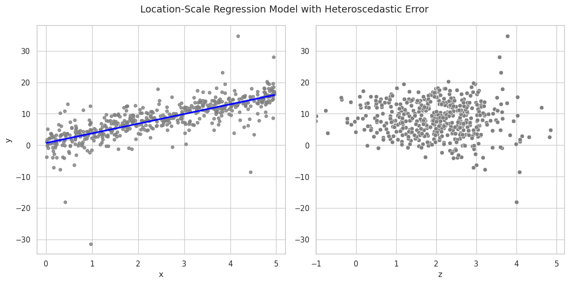
The simulated data displays a linear relationship between the response \(\mathbf{y}\) and the covariate \(\mathbf{x}\). The slope of the estimated regression line is close to the true \(\beta_1 = 3\). The right plot shows the relationship between \(\mathbf{y}\) and the scale covariate vector \(\mathbf{z}\). Larger values of \(\mathbf{ z}\) lead to a larger variance of the response.
fig, (ax1, ax2) = plt.subplots(nrows=1, ncols=2, figsize=(12, 6))
sns.regplot(
    x=X_mat[:, 1],
    y=y_vec,
    fit_reg=True,
    scatter_kws=dict(color="grey", s=20),
    line_kws=dict(color="blue"),
    ax=ax1,
).set(xlabel="x", ylabel="y", xlim=[-0.2, 5.2])

sns.scatterplot(
    x=Z_mat[:, 1],
    y=y_vec,
    color="grey",
    s=40,
    ax=ax2,
).set(xlabel="z", xlim=[-1, 5.2])

fig.suptitle("Location-Scale Regression Model with Heteroscedastic Error")
fig.tight_layout()
plt.show()
Since positivity of the scale is ensured by the exponential function,
the linear part \(\mathbf{z}_i^T \boldsymbol{\gamma}\) is not restricted
to the positive real line. Hence, setting a normal prior distribution
for \(\gamma\) is feasible, leading to an almost symmetric specification
of the location and scale parts of the model. The variables beta and
gamma are initialized as parameter variables with weakly informative
normal priors. We also attach MCMCSpec objects that
tell LieselMCMC to sample each parameter block with a NUTS
kernel:
dist_beta = lsl.Dist(tfd.Normal, loc=0.0, scale=100.0)
beta = lsl.Var.new_param(
    jnp.array([10.0, 10.0]),
    dist_beta,
    name="beta",
    inference=gs.MCMCSpec(gs.NUTSKernel),
)

dist_gamma = lsl.Dist(tfd.Normal, loc=0.0, scale=100.0)
gamma = lsl.Var.new_param(
    jnp.array([5.0, 5.0]),
    dist_gamma,
    name="gamma",
    inference=gs.MCMCSpec(gs.NUTSKernel),
)
The additional complexity of the location-scale model compared to the
standard linear model is handled in the next step. Since gamma takes
values on the whole real line, but the response variable y expects a
positive scale input, we apply the exponential function to the scale
predictor. The mean predictor mu and the positive scale are then
passed to the normal likelihood of y.
X = lsl.Var.new_obs(X_mat, name="X")
Z = lsl.Var.new_obs(Z_mat, name="Z")

mu = lsl.Var(lsl.Calc(jnp.dot, X, beta), name="mu")

log_scale = lsl.Calc(jnp.dot, Z, gamma)
scale = lsl.Var(lsl.Calc(jnp.exp, log_scale), name="scale")

dist_y = lsl.Dist(tfd.Normal, loc=mu, scale=scale)
y = lsl.Var.new_obs(y_vec, dist_y, name="y")
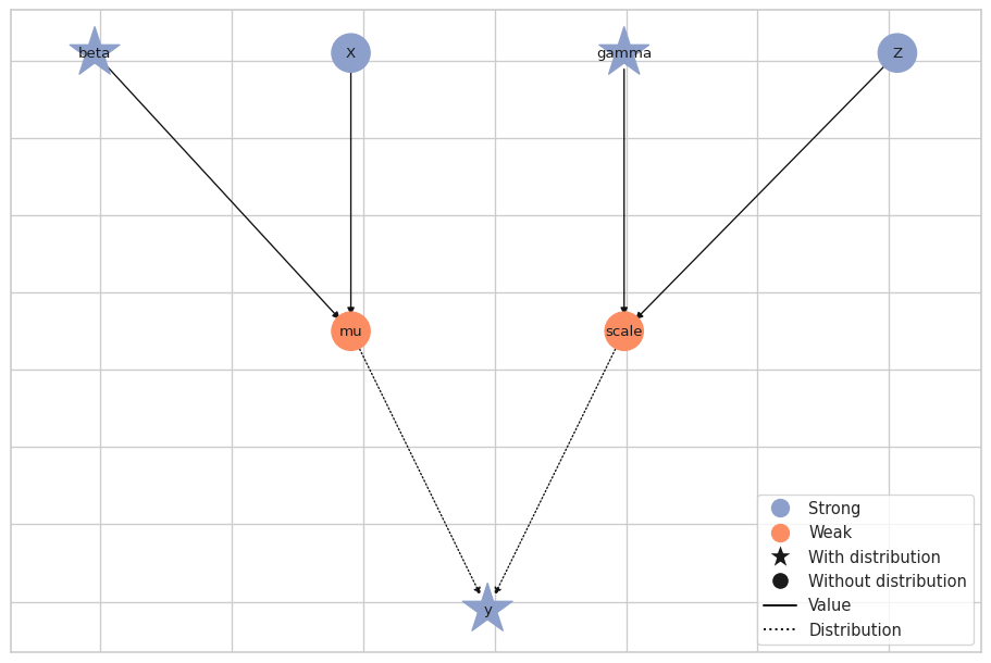
We can now initialize the model from the response variable and visualize
the resulting graph. All other variables are collected automatically
because they are inputs to y, directly or indirectly.
model = lsl.Model(y)

model.plot(width=12, height=8)
We generate posterior samples with the No-U-Turn sampler. The sampler
setup is taken from the inference specifications on beta and gamma,
so LieselMCMC can construct the two NUTS kernels directly from
the model. We run 1000 adaptation iterations and then draw 1000
posterior samples per chain.
results = gs.LieselMCMC(model).run_for_epochs(
    seed=1, num_chains=4, adaptation=1000, posterior=1000
)
liesel.goose.builder - WARNING - No jitter functions provided for position keys 'beta', 'gamma'. The initial values for these keys won't be jittered
liesel.goose.engine - INFO - Initializing kernels...
liesel.goose.engine - INFO - Done
liesel.goose.engine - INFO - Starting epoch: FAST_ADAPTATION, 100 transitions, 25 jitted together

  0%|                                                  | 0/4 [00:00<?, ?chunk/s]
 25%|██████████▌                               | 1/4 [00:04<00:14,  4.92s/chunk]
100%|██████████████████████████████████████████| 4/4 [00:04<00:00,  1.23s/chunk]
liesel.goose.engine - WARNING - Errors per chain for kernel_00: 5, 5, 3, 4 / 100 transitions
liesel.goose.engine - WARNING - Errors per chain for kernel_01: 5, 6, 5, 7 / 100 transitions
liesel.goose.engine - INFO - Finished epoch
liesel.goose.engine - INFO - Starting epoch: SLOW_ADAPTATION, 25 transitions, 25 jitted together

  0%|                                                  | 0/1 [00:00<?, ?chunk/s]
100%|█████████████████████████████████████████| 1/1 [00:00<00:00, 614.91chunk/s]
liesel.goose.engine - WARNING - Errors per chain for kernel_00: 1, 1, 2, 1 / 25 transitions
liesel.goose.engine - WARNING - Errors per chain for kernel_01: 2, 1, 2, 1 / 25 transitions
liesel.goose.engine - INFO - Finished epoch
liesel.goose.engine - INFO - Starting epoch: SLOW_ADAPTATION, 50 transitions, 25 jitted together

  0%|                                                  | 0/2 [00:00<?, ?chunk/s]
100%|████████████████████████████████████████| 2/2 [00:00<00:00, 1233.62chunk/s]
liesel.goose.engine - WARNING - Errors per chain for kernel_00: 1, 2, 3, 2 / 50 transitions
liesel.goose.engine - WARNING - Errors per chain for kernel_01: 2, 3, 1, 2 / 50 transitions
liesel.goose.engine - INFO - Finished epoch
liesel.goose.engine - INFO - Starting epoch: SLOW_ADAPTATION, 100 transitions, 25 jitted together

  0%|                                                  | 0/4 [00:00<?, ?chunk/s]
100%|████████████████████████████████████████| 4/4 [00:00<00:00, 1136.82chunk/s]
liesel.goose.engine - WARNING - Errors per chain for kernel_00: 2, 2, 0, 1 / 100 transitions
liesel.goose.engine - WARNING - Errors per chain for kernel_01: 2, 2, 1, 2 / 100 transitions
liesel.goose.engine - INFO - Finished epoch
liesel.goose.engine - INFO - Starting epoch: SLOW_ADAPTATION, 525 transitions, 25 jitted together

  0%|                                                 | 0/21 [00:00<?, ?chunk/s]
 76%|█████████████████████████████▋         | 16/21 [00:00<00:00, 148.20chunk/s]
100%|███████████████████████████████████████| 21/21 [00:00<00:00, 137.08chunk/s]
liesel.goose.engine - WARNING - Errors per chain for kernel_00: 2, 5, 6, 2 / 525 transitions
liesel.goose.engine - WARNING - Errors per chain for kernel_01: 4, 5, 3, 3 / 525 transitions
liesel.goose.engine - INFO - Finished epoch
liesel.goose.engine - INFO - Starting epoch: FAST_ADAPTATION, 200 transitions, 25 jitted together

  0%|                                                  | 0/8 [00:00<?, ?chunk/s]
100%|█████████████████████████████████████████| 8/8 [00:00<00:00, 424.61chunk/s]
liesel.goose.engine - WARNING - Errors per chain for kernel_00: 0, 2, 4, 3 / 200 transitions
liesel.goose.engine - WARNING - Errors per chain for kernel_01: 3, 6, 4, 1 / 200 transitions
liesel.goose.engine - INFO - Finished epoch
liesel.goose.engine - INFO - Finished warmup
liesel.goose.engine - INFO - Starting epoch: POSTERIOR, 1000 transitions, 25 jitted together

  0%|                                                 | 0/40 [00:00<?, ?chunk/s]
 45%|█████████████████▌                     | 18/40 [00:00<00:00, 174.41chunk/s]
 90%|███████████████████████████████████    | 36/40 [00:00<00:00, 126.30chunk/s]
100%|███████████████████████████████████████| 40/40 [00:00<00:00, 129.15chunk/s]
liesel.goose.engine - INFO - Finished epoch
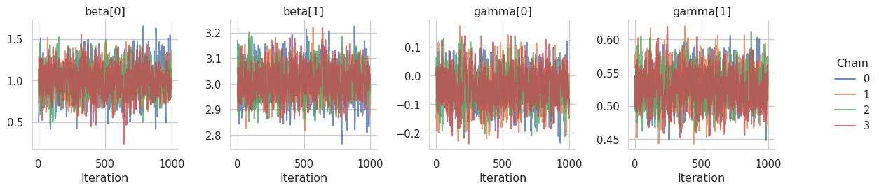
Now that we have 1000 posterior samples per chain, we can check the results, starting with trace plots for the sampled parameters.
gs.plot_trace(results, ncol=4)