Bayesian Measurement Error Correction#
In this tutorial, we implement a regression model with Bayesian measurement error correction in Liesel. The model should capture the effect of a continuous covariate \(x\), which is assumed to be affected by measurement error. We further want to estimate the posterior distribution of the model parameters and the latent covariate.
Measurement Error#
Assuming a total number of \(M\) replicates of the covariate \(x\) affected by measurement error, we can write the measurement error model as
In this tutorial, the replicates are assumed to be independent with constant variance
The fundamental concept behind Bayesian measurement error correction is to treat the true, unknown covariate values \(x_i\) as additional latent variables. These values are then imputed using MCMC simulations while simultaneously estimating all other parameters of the model. To achieve this, we assign a simple prior distribution to \(x_i\). We further add hyperpriors with assigned prior distributions to the distribution parameters of \(x_i\), to achieve further flexibility.
Imports#
First, we import all of the required packages.
import jax
import jax.numpy as jnp
import liesel.model as lsl
import liesel.goose as gs
import liesel.contrib.splines as splines
import tensorflow_probability.substrates.jax as tfp
import tensorflow_probability.substrates.jax.bijectors as tfb
import numpy as np
import matplotlib.pyplot as plt
import seaborn as sns

from liesel.contrib.splines import equidistant_knots, basis_matrix
from liesel.distributions.mvn_degen import MultivariateNormalDegenerate

tfd = tfp.distributions
Data#
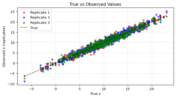
Afterwards we will start by simulating some data with replicates.
# Define the number of samples and replicates
seed = 123

n = 500  # Number of data points
M = 3  # Number of replicates per sample
key = jax.random.PRNGKey(seed)
x = 10 + 5 * jax.random.normal(key, n)  # create the true x

sigma_u_true = 1  # variance of the replicates

keys = jax.random.split(key, n)
x_tilde = jnp.array([
    x[i] + sigma_u_true * jax.random.normal(keys[i], (M,)) for i in range(n)
])  # observed x-values
# Plot Data
fig, ax1 = plt.subplots(figsize=(8, 4))

# True x vs observed replicates
ax1.scatter(x, x_tilde[:, 0], alpha=0.6, s=20, label="Replicate 1", color="red")
ax1.scatter(x, x_tilde[:, 1], alpha=0.6, s=20, label="Replicate 2", color="blue")
ax1.scatter(x, x_tilde[:, 2], alpha=0.6, s=20, label="Replicate 3", color="green")
ax1.plot([x.min(), x.max()], [x.min(), x.max()], "k--", alpha=0.7, label="True")
ax1.set_xlabel("True x")
ax1.set_ylabel("Observed x (replicates)")
ax1.set_title("True vs Observed Values")
ax1.legend()
ax1.grid(True, alpha=0.3)
We simulate the response as done in the linear regression tutorial from the model \(y_i | x_i \sim \mathcal{N}(\beta_0 + \beta_1 x_i, \;\sigma^{2}_y)\) given our true covariate.
rng = np.random.default_rng(42)

sigma_y_true = 1.0  # variance of the response

true_beta = np.array([1.0, 2.0])

X_mat_true = np.column_stack([np.ones(n), x])

eps = rng.normal(scale=sigma_y_true, size=n)
y_vec = X_mat_true @ true_beta + eps
Implementing the Model in Liesel#
Now that we have our data we can define our distributions from above in
Liesel, setting \(\tau^2_{\mu} = 1000\) and \(a_x = b_x = 0.001\). We will
initialize \(x\) using the mean of our observed measurements. We also need
to assign a normal distribution to the observed measurements and define
\(\sigma^{2}_u\) (the variance of the measurements). Note that we are
building a hierarchical model by providing a Var instance for
the loc and scale arguments of the different distributions.
We begin by establishing \(\tau^2_{x}\).
# Define hyperparameters for variance of x
a_x = lsl.Var.new_param(0.001, name="a_x")
b_x = lsl.Var.new_param(0.001, name="b_x")

# Define prior for tau2_x using an Inverse Gamma distribution
tau2_x_prior = lsl.Dist(tfd.InverseGamma, concentration=a_x, scale=b_x)
tau2_x = lsl.Var.new_param(10.0, distribution=tau2_x_prior, name="tau2_x")
Following that we define \(\tau^2_{\mu}\), so we can define \(\mu_x\) afterwards.
# Define the scales for mu_x (mean of x)
tau2_mu = lsl.Var.new_param(1000.0, name="tau2_mu")

# Define prior for mu_x using a Normal distribution
mu_x_prior = lsl.Dist(tfd.Normal, loc=0.0, scale=tau2_mu)

# Define mu_x as a parameter with the prior distribution
mu_x = lsl.Var.new_param(x_tilde.mean(), distribution=mu_x_prior, name="mu_x")
With that we then can configure the prior distribution for \(x_i\) and construct our x-values as a model parameter.
# Define prior distribution for x
x_prior_dist = lsl.Dist(tfd.Normal, loc=mu_x, scale=tau2_x)

# Estimate x using the mean of replicates and assign a prior distribution
x_estimated = lsl.Var.new_param(
    x_tilde.mean(axis=1),  # initial estimation is the mean of the replicates
    distribution=x_prior_dist,
    name="x_estimated",
)
Now, we incorporate the variance and scale of our measurements and formalize the likelihood.
# Define the scale of the measurement distribution
sigma_u_prior = lsl.Dist(tfd.InverseGamma, concentration=0.01, scale=0.01)
sigma_sq_u = lsl.Var.new_param(
    value=10.0, distribution=sigma_u_prior, name="sigma_sq_u"
)
sigma_u = lsl.Var.new_calc(jnp.sqrt, sigma_sq_u, name="sigma_u").update()
log_sigma_u = sigma_sq_u.transform(tfb.Exp())


# Measurement distribution location
measurement_dist_loc = lsl.Calc(lambda x: jnp.expand_dims(x, -1), x_estimated)

# Define likelihood model for measurement error
measurement_dist = lsl.Dist(tfd.Normal, loc=measurement_dist_loc, scale=sigma_u)
# Measurements
x_tilde_var = lsl.Var(x_tilde, distribution=measurement_dist, name="x_tilde")
Afterwards we define \(\boldsymbol{\beta}\), our design matrix and
\(\sigma^{2}_y\) (the variance of the response). Note that we have to
create the design matrix using Var.new_calc() as we continuously
update our x-values during the inference.
beta_prior = lsl.Dist(tfd.Normal, loc=0.0, scale=100.0)
beta = lsl.Var.new_param(np.array([0.0, 0.0]), name="beta", distribution=beta_prior)


def create_x(x):
    return jnp.column_stack([np.ones(n), x])


X_mat = lsl.Var.new_calc(create_x, x_estimated, name="X")  # design matrix

a = lsl.Var.new_param(0.01, name="a")
b = lsl.Var.new_param(0.01, name="b")

sigma_sq_prior = lsl.Dist(tfd.InverseGamma, concentration=a, scale=b)
sigma_sq_y = lsl.Var.new_param(
    value=10.0, distribution=sigma_sq_prior, name="sigma_sq_y"
)
sigma_y = lsl.Var.new_calc(jnp.sqrt, sigma_sq_y, name="sigma_y").update()
log_sigma = sigma_sq_y.transform(tfb.Exp())
We now can create the distribution for our response. Note that the response is assumed to be distributed as \(y_i | \tilde{x}_i \sim \mathcal{N}(\beta_0 + \beta_1 x_i, \;\sigma^{2}_y)\) as we are estimating the x-values as well. Both \(\sigma^{2}_y\) (variance of the response) and \(\sigma^{2}_u\) (variance of the measurements) are assumed to follow an \(\text{InverseGamma}(a, b)\) distribution and are log-transformed to ensure positivity.
# create joint model for x and y

mu_of_y = lsl.Var.new_calc(  # compute the dot product
    jnp.dot, X_mat, beta, name="mu_of_y"
)

# Define the likelihood distribution of y (Normal with estimated mean and scale)
y_dist = lsl.Dist(tfd.Normal, loc=mu_of_y, scale=sigma_y)

# Define y as an observed variable with the specified distribution
y_var = lsl.Var.new_obs(value=y_vec, distribution=y_dist, name="y")
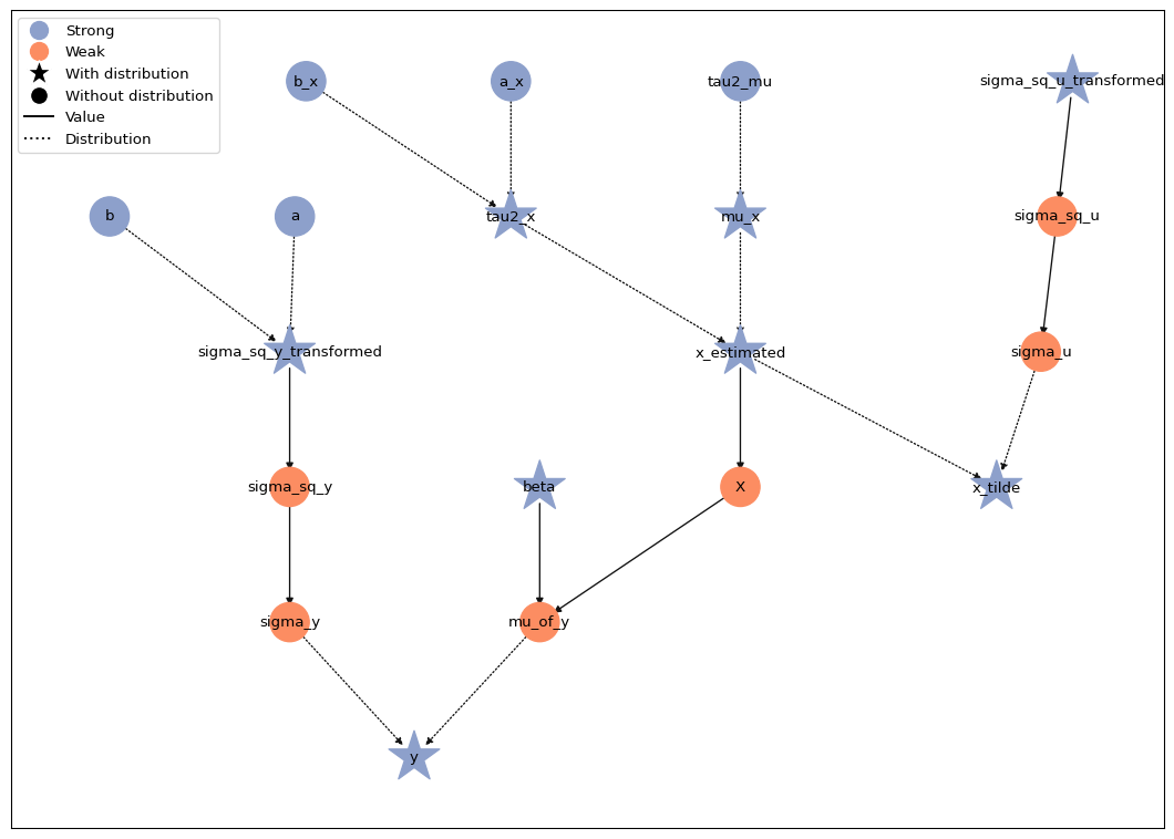
Now we can take a look at our model
# create joint model for x and y
model = lsl.Model([y_var, x_tilde_var])

# Plot tree
model.plot_vars()
liesel.model.model - WARNING - Inconsistent log prob decomposition: Model.log_prob=-19741.52 ≠ (Model.log_lik=-14871.53 + Model.log_prior=-1715.54).
liesel.model.model - WARNING - Var(name="x_tilde") has a distribution but Var.parameter=False and Var.observed=False.
MCMC Inference#
We choose NUTS kernels (NUTSKernel) for generating
posterior samples of \(\sigma_y\), \(\sigma_u\), \(\boldsymbol{\beta}\), and
to sample our x-values. To draw from \(\mu_x\) and \(\tau^2_x\) we use Gibbs
kernels (GibbsKernel), as this allows us to use custom
transition functions for our parameters. The full conditionals are:
Let us implement these
def transition_mu_x(prng_key, model_state):
    """
    Sample mu_x from its posterior distribution conditioned on the data.

    Args:
        prng_key: The random number generator key for sampling.
        model_state: A dictionary containing the model parameters and state.

    Returns:
        dict: A dictionary containing the sampled mu_x.
    """
    # Extract relevant parameters from model state
    pos = interface.extract_position(
        position_keys=["x_estimated", "tau2_x", "tau2_mu", "a_x", "b_x"],
        model_state=model_state,
    )
    x = pos["x_estimated"]
    n = len(x)
    tau2_mu = pos["tau2_mu"]
    tau2_x = pos["tau2_x"]
    a_x = pos["a_x"]
    b_x = pos["b_x"]

    # Compute the posterior mean and standard deviation for mu_x
    normal_sample = jax.random.normal(prng_key, (1,))
    mu_mean = (n * jnp.mean(x) * tau2_mu) / (n * tau2_mu + tau2_x)
    mu_std = jnp.sqrt(tau2_x * tau2_mu / (n * tau2_mu + tau2_x))

    # Sample mu_x from a normal distribution
    mu_x = jnp.squeeze(mu_mean + mu_std * normal_sample)

    return {"mu_x": mu_x}


def transition_tau2_x(prng_key, model_state):
    """
    Sample tau2_x from its posterior distribution using the inverse gamma distribution.

    Args:
        prng_key: The random number generator key for sampling.
        model_state: A dictionary containing the model parameters and state.

    Returns:
        dict: A dictionary containing the sampled tau2_x.
    """
    # Extract relevant parameters from model state
    pos = interface.extract_position(
        position_keys=["a_x", "b_x", "x_estimated", "mu_x", "b_x"],
        model_state=model_state,
    )
    a_x = pos["a_x"]
    b_x = pos["b_x"]
    x = pos["x_estimated"]
    n = len(x)
    mu_x = pos["mu_x"]

    # Compute the new alpha and beta for the inverse gamma distribution
    alpha_new = a_x + n / 2
    beta_new = b_x + ((x - mu_x) ** 2).sum() / 2

    # Sample tau2_x from the inverse gamma distribution
    tau2_x = jnp.squeeze(
        tfd.InverseGamma(concentration=alpha_new, scale=beta_new).sample(seed=prng_key)
    )

    return {"tau2_x": tau2_x}
We set up our engine and draw 2000 posterior samples.
# #add kernels and return engine
interface = gs.LieselInterface(model)
eb_sample = gs.EngineBuilder(seed=2, num_chains=4)
eb_sample.set_model(gs.LieselInterface(model))
eb_sample.set_initial_values(model.state)


eb_sample.add_kernel(gs.NUTSKernel(["x_estimated"]))

eb_sample.add_kernel(gs.GibbsKernel(["mu_x"], transition_mu_x))
eb_sample.add_kernel(gs.GibbsKernel(["tau2_x"], transition_tau2_x))

eb_sample.add_kernel(gs.NUTSKernel(["beta"]))
eb_sample.add_kernel(gs.NUTSKernel(["sigma_sq_y_transformed"]))
eb_sample.add_kernel(gs.NUTSKernel(["sigma_sq_u_transformed"]))

eb_sample.set_duration(
    warmup_duration=1000,
    posterior_duration=2000,
    thinning_posterior=1,
    term_duration=200,
)

engine = eb_sample.build()
engine.sample_all_epochs()
liesel.goose.builder - WARNING - No jitter functions provided. The initial values won't be jittered
liesel.goose.engine - INFO - Initializing kernels...
liesel.goose.engine - INFO - Done
liesel.goose.engine - INFO - Starting epoch: FAST_ADAPTATION, 75 transitions, 25 jitted together

  0%|                                                  | 0/3 [00:00<?, ?chunk/s]
 33%|██████████████                            | 1/3 [00:11<00:22, 11.32s/chunk]
100%|██████████████████████████████████████████| 3/3 [00:11<00:00,  3.78s/chunk]
liesel.goose.engine - WARNING - Errors per chain for kernel_00: 0, 1, 1, 0 / 75 transitions
liesel.goose.engine - WARNING - Errors per chain for kernel_03: 2, 6, 2, 3 / 75 transitions
liesel.goose.engine - WARNING - Errors per chain for kernel_04: 4, 3, 6, 2 / 75 transitions
liesel.goose.engine - WARNING - Errors per chain for kernel_05: 2, 2, 3, 4 / 75 transitions
liesel.goose.engine - INFO - Finished epoch
liesel.goose.engine - INFO - Starting epoch: SLOW_ADAPTATION, 25 transitions, 25 jitted together

  0%|                                                  | 0/1 [00:00<?, ?chunk/s]
100%|█████████████████████████████████████████| 1/1 [00:00<00:00, 501.95chunk/s]
liesel.goose.engine - WARNING - Errors per chain for kernel_00: 1, 2, 1, 1 / 25 transitions
liesel.goose.engine - WARNING - Errors per chain for kernel_03: 1, 2, 1, 2 / 25 transitions
liesel.goose.engine - WARNING - Errors per chain for kernel_04: 1, 2, 1, 1 / 25 transitions
liesel.goose.engine - WARNING - Errors per chain for kernel_05: 1, 1, 2, 1 / 25 transitions
liesel.goose.engine - INFO - Finished epoch
liesel.goose.engine - INFO - Starting epoch: SLOW_ADAPTATION, 50 transitions, 25 jitted together

  0%|                                                  | 0/2 [00:00<?, ?chunk/s]
100%|█████████████████████████████████████████| 2/2 [00:00<00:00, 664.39chunk/s]
liesel.goose.engine - WARNING - Errors per chain for kernel_00: 1, 1, 1, 1 / 50 transitions
liesel.goose.engine - WARNING - Errors per chain for kernel_03: 1, 2, 1, 3 / 50 transitions
liesel.goose.engine - WARNING - Errors per chain for kernel_04: 3, 1, 2, 1 / 50 transitions
liesel.goose.engine - WARNING - Errors per chain for kernel_05: 2, 1, 2, 1 / 50 transitions
liesel.goose.engine - INFO - Finished epoch
liesel.goose.engine - INFO - Starting epoch: SLOW_ADAPTATION, 100 transitions, 25 jitted together

  0%|                                                  | 0/4 [00:00<?, ?chunk/s]
100%|████████████████████████████████████████| 4/4 [00:00<00:00, 1001.45chunk/s]
liesel.goose.engine - WARNING - Errors per chain for kernel_00: 1, 1, 1, 1 / 100 transitions
liesel.goose.engine - WARNING - Errors per chain for kernel_03: 3, 3, 3, 2 / 100 transitions
liesel.goose.engine - WARNING - Errors per chain for kernel_04: 3, 3, 1, 1 / 100 transitions
liesel.goose.engine - WARNING - Errors per chain for kernel_05: 2, 1, 2, 2 / 100 transitions
liesel.goose.engine - INFO - Finished epoch
liesel.goose.engine - INFO - Starting epoch: SLOW_ADAPTATION, 550 transitions, 25 jitted together

  0%|                                                 | 0/22 [00:00<?, ?chunk/s]
 41%|████████████████▊                        | 9/22 [00:00<00:00, 70.20chunk/s]
 77%|██████████████████████████████▉         | 17/22 [00:00<00:00, 31.30chunk/s]
100%|████████████████████████████████████████| 22/22 [00:00<00:00, 27.77chunk/s]
100%|████████████████████████████████████████| 22/22 [00:00<00:00, 30.68chunk/s]
liesel.goose.engine - WARNING - Errors per chain for kernel_00: 1, 1, 1, 1 / 550 transitions
liesel.goose.engine - WARNING - Errors per chain for kernel_03: 2, 3, 5, 6 / 550 transitions
liesel.goose.engine - WARNING - Errors per chain for kernel_04: 3, 3, 3, 4 / 550 transitions
liesel.goose.engine - WARNING - Errors per chain for kernel_05: 2, 4, 3, 1 / 550 transitions
liesel.goose.engine - INFO - Finished epoch
liesel.goose.engine - INFO - Starting epoch: FAST_ADAPTATION, 200 transitions, 25 jitted together

  0%|                                                  | 0/8 [00:00<?, ?chunk/s]
100%|██████████████████████████████████████████| 8/8 [00:00<00:00, 98.67chunk/s]
liesel.goose.engine - WARNING - Errors per chain for kernel_00: 1, 1, 1, 1 / 200 transitions
liesel.goose.engine - WARNING - Errors per chain for kernel_03: 1, 3, 5, 3 / 200 transitions
liesel.goose.engine - WARNING - Errors per chain for kernel_04: 1, 1, 0, 2 / 200 transitions
liesel.goose.engine - WARNING - Errors per chain for kernel_05: 1, 2, 2, 2 / 200 transitions
liesel.goose.engine - INFO - Finished epoch
liesel.goose.engine - INFO - Finished warmup
liesel.goose.engine - INFO - Starting epoch: POSTERIOR, 2000 transitions, 25 jitted together

  0%|                                                 | 0/80 [00:00<?, ?chunk/s]
 12%|█████                                   | 10/80 [00:00<00:00, 86.03chunk/s]
 24%|█████████▌                              | 19/80 [00:00<00:01, 38.29chunk/s]
 31%|████████████▌                           | 25/80 [00:00<00:01, 33.27chunk/s]
 38%|███████████████                         | 30/80 [00:00<00:01, 30.89chunk/s]
 42%|█████████████████                       | 34/80 [00:01<00:01, 29.61chunk/s]
 48%|███████████████████                     | 38/80 [00:01<00:01, 28.63chunk/s]
 51%|████████████████████▌                   | 41/80 [00:01<00:01, 28.11chunk/s]
 55%|██████████████████████                  | 44/80 [00:01<00:01, 27.65chunk/s]
 59%|███████████████████████▌                | 47/80 [00:01<00:01, 27.27chunk/s]
 62%|█████████████████████████               | 50/80 [00:01<00:01, 26.98chunk/s]
 66%|██████████████████████████▌             | 53/80 [00:01<00:01, 26.83chunk/s]
 70%|████████████████████████████            | 56/80 [00:01<00:00, 26.70chunk/s]
 74%|█████████████████████████████▌          | 59/80 [00:01<00:00, 26.51chunk/s]
 78%|███████████████████████████████         | 62/80 [00:02<00:00, 26.36chunk/s]
 81%|████████████████████████████████▌       | 65/80 [00:02<00:00, 26.41chunk/s]
 85%|██████████████████████████████████      | 68/80 [00:02<00:00, 25.89chunk/s]
 89%|███████████████████████████████████▌    | 71/80 [00:02<00:00, 25.91chunk/s]
 92%|█████████████████████████████████████   | 74/80 [00:02<00:00, 26.02chunk/s]
 96%|██████████████████████████████████████▌ | 77/80 [00:02<00:00, 25.15chunk/s]
100%|████████████████████████████████████████| 80/80 [00:02<00:00, 25.54chunk/s]
100%|████████████████████████████████████████| 80/80 [00:02<00:00, 28.65chunk/s]
liesel.goose.engine - INFO - Finished epoch
Now we can take a look at the results for our parameters
results = engine.get_results()
summary = gs.Summary(results)
gs.Summary(results, deselected=["x_estimated"])
Parameter summary:
|
kernel |
mean |
sd |
q_0.05 |
q_0.5 |
q_0.95 |
sample_size |
ess_bulk |
ess_tail |
rhat |
||
|---|---|---|---|---|---|---|---|---|---|---|---|
|
parameter |
index |
||||||||||
|
beta |
(0,) |
kernel_03 |
1.241 |
0.151 |
0.995 |
1.240 |
1.489 |
8000 |
569.091 |
933.972 |
1.007 |
|
(1,) |
kernel_03 |
1.975 |
0.013 |
1.953 |
1.975 |
1.997 |
8000 |
649.981 |
1004.927 |
1.006 |
|
|
mu_x |
() |
kernel_01 |
10.070 |
0.235 |
9.686 |
10.071 |
10.457 |
8000 |
7337.531 |
7434.558 |
1.000 |
|
sigma_sq_u_transformed |
() |
kernel_05 |
-0.015 |
0.046 |
-0.089 |
-0.016 |
0.059 |
8000 |
1371.552 |
2384.836 |
1.001 |
|
sigma_sq_y_transformed |
() |
kernel_04 |
0.019 |
0.158 |
-0.254 |
0.029 |
0.262 |
8000 |
386.460 |
590.875 |
1.008 |
|
tau2_x |
() |
kernel_02 |
27.401 |
1.773 |
24.666 |
27.308 |
30.402 |
8000 |
7908.989 |
7676.281 |
1.000 |
Acceptance probabilities:
|
acceptance_probability |
position_moved |
|||
|---|---|---|---|---|
|
kernel |
positions |
phase |
||
|
kernel_00 |
x_estimated |
posterior |
0.811 |
NaN |
|
warmup |
0.791 |
NaN |
||
|
kernel_01 |
mu_x |
posterior |
1.000 |
1.000 |
|
warmup |
1.000 |
1.000 |
||
|
kernel_02 |
tau2_x |
posterior |
1.000 |
1.000 |
|
warmup |
1.000 |
1.000 |
||
|
kernel_03 |
beta |
posterior |
0.887 |
NaN |
|
warmup |
0.791 |
NaN |
||
|
kernel_04 |
sigma_sq_y_transformed |
posterior |
0.878 |
NaN |
|
warmup |
0.792 |
NaN |
||
|
kernel_05 |
sigma_sq_u_transformed |
posterior |
0.882 |
NaN |
|
warmup |
0.791 |
NaN |
Error summary:
|
count |
sample_size |
sample_size_total |
relative |
|||||
|---|---|---|---|---|---|---|---|---|
|
kernel |
positions |
error_code |
error_msg |
phase |
||||
|
kernel_00 |
x_estimated |
1 |
divergent transition |
warmup |
22 |
4000 |
4000 |
0.005 |
|
posterior |
0 |
8000 |
8000 |
0.000 |
||||
|
2 |
maximum tree depth |
warmup |
1 |
4000 |
4000 |
0.000 |
||
|
posterior |
0 |
8000 |
8000 |
0.000 |
||||
|
kernel_03 |
beta |
1 |
divergent transition |
warmup |
65 |
4000 |
4000 |
0.016 |
|
posterior |
0 |
8000 |
8000 |
0.000 |
||||
|
kernel_04 |
sigma_sq_y_transformed |
1 |
divergent transition |
warmup |
52 |
4000 |
4000 |
0.013 |
|
posterior |
0 |
8000 |
8000 |
0.000 |
||||
|
kernel_05 |
sigma_sq_u_transformed |
1 |
divergent transition |
warmup |
46 |
4000 |
4000 |
0.012 |
|
posterior |
0 |
8000 |
8000 |
0.000 |
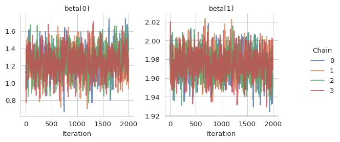
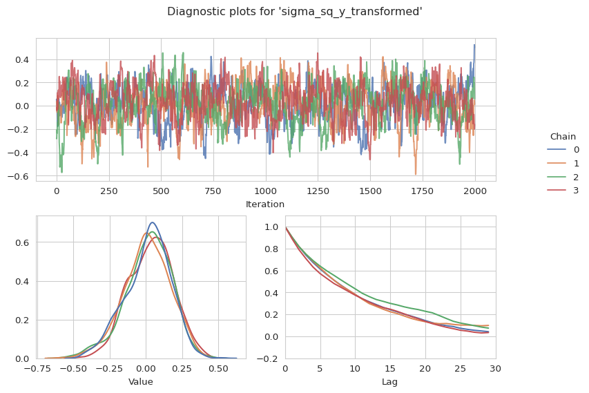
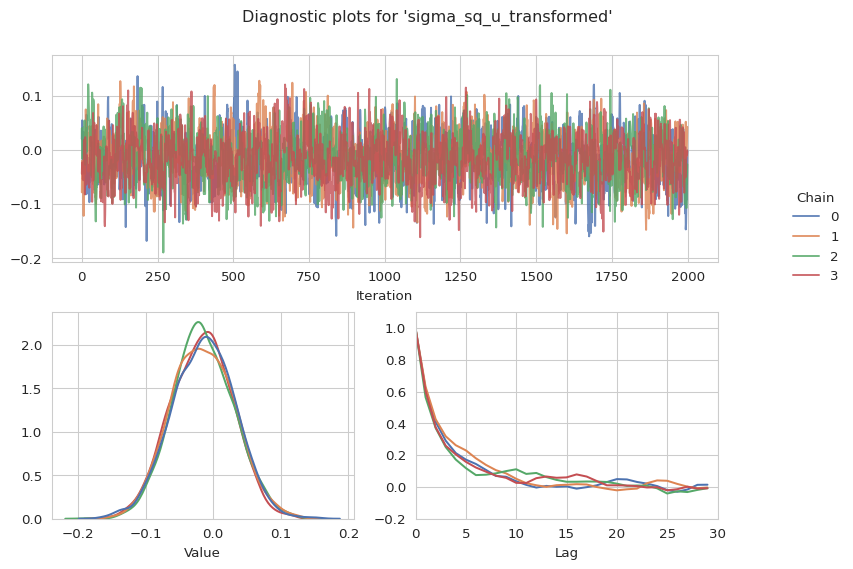
And the traceplots for \(\beta\), \(\log(\sigma_y)\) and \(\log(\sigma_u)\).
# Plot the trace of all location coefficients
gs.plot_trace(results, "beta")
gs.plot_param(results, "sigma_sq_y_transformed")
gs.plot_param(results, "sigma_sq_u_transformed")
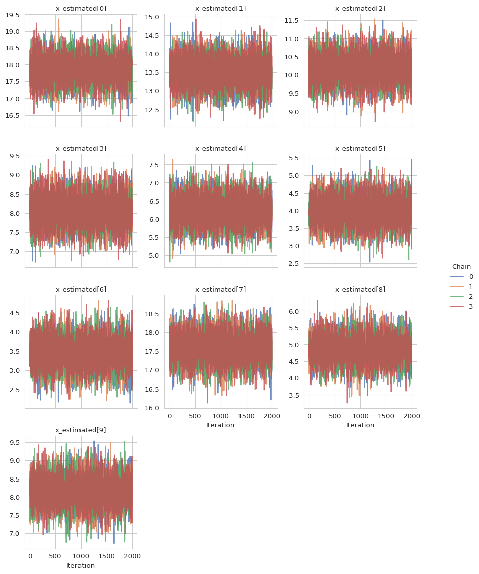
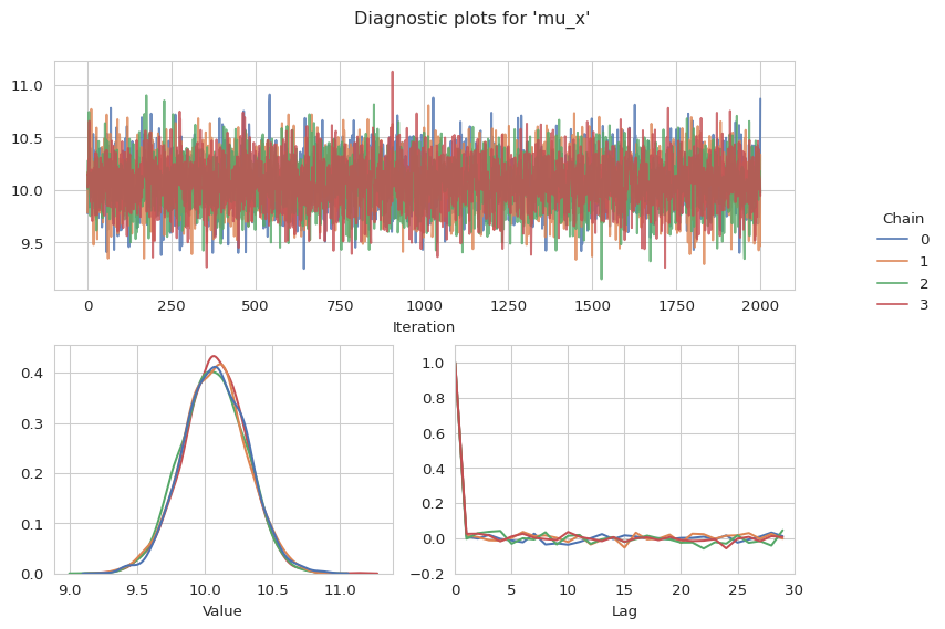
We further can also have a look at our first ten sampled x values and the mean
gs.plot_trace(results, "x_estimated", range(10))
gs.plot_param(results, "mu_x")
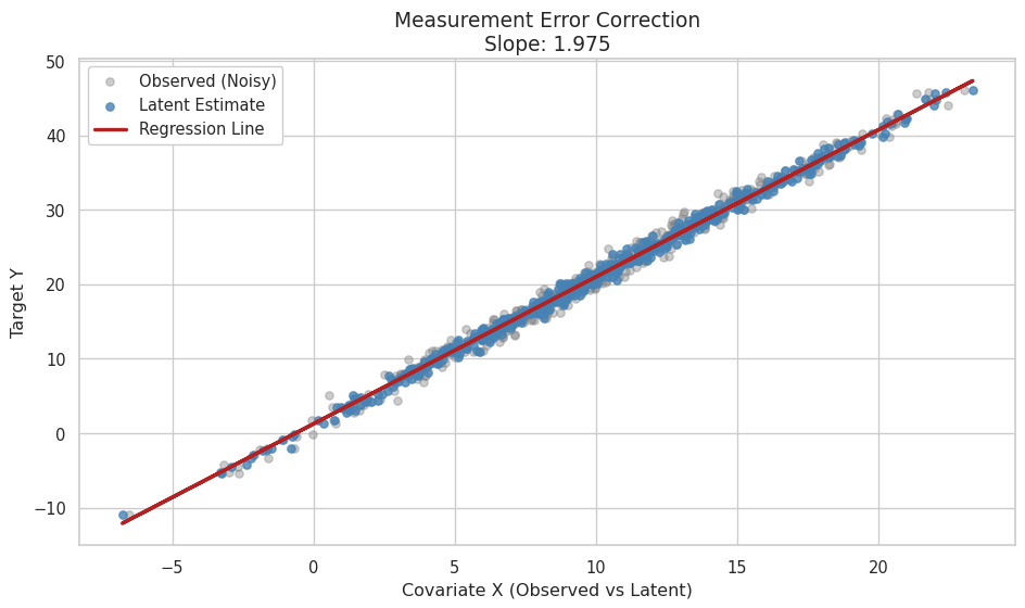
To finally evaluate the model we can plot the regression line
# Extract quantities from the summary
x_means = summary.quantities["mean"]["x_estimated"]
beta_est = summary.quantities["mean"]["beta"]
y_pred = beta_est[0] + beta_est[1] * x_means

sns.set_theme(style="whitegrid")

fig, ax = plt.subplots(figsize=(10, 6))

# Plot Observed Data (Faint)
ax.scatter(x, y_vec, color="gray", alpha=0.4, s=30, label="Observed (Noisy)")

# Plot Estimated Latent Positions (Stronger)
ax.scatter(x_means, y_vec, color="steelblue", alpha=0.8, s=30, label="Latent Estimate")

# Plot Regression Line
ax.plot(x_means, y_pred, color="firebrick", lw=2.5, label="Regression Line")

# Labels and Title
ax.set_title(f"Measurement Error Correction\nSlope: {beta_est[1]:.3f}", fontsize=14)
ax.set_xlabel("Covariate X (Observed vs Latent)", fontsize=12)
ax.set_ylabel("Target Y", fontsize=12)
ax.legend(frameon=True, fancybox=True, framealpha=1, loc="best")

plt.tight_layout()
plt.show()