Linear Regression#

In this tutorial, we build a linear regression model with Liesel and estimate it with Goose. Our goal is to illustrate the most fundamental features of the software in a straight-forward context.

Imports#

Before we can generate the data and build the model, we need to load Liesel and a number of other packages. We usually import the model building library liesel.model as lsl, and the MCMC library liesel.goose as gs.

import jax
import jax.numpy as jnp
import numpy as np

# We use distributions and bijectors from tensorflow probability
import tensorflow_probability.substrates.jax.distributions as tfd
import tensorflow_probability.substrates.jax.bijectors as tfb

import liesel.goose as gs
import liesel.model as lsl

import matplotlib.pyplot as plt

Generating the data#

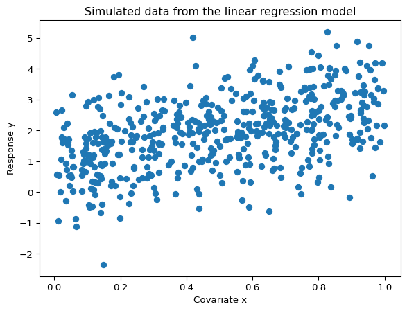
Now we can simulate 500 observations from the linear regression model \(y_i \sim \mathcal{N}(\beta_0 + \beta_1 x_i, \;\sigma^2)\) with the true parameters \(\boldsymbol{\beta} = (\beta_0, \beta_1)' = (1, 2)'\) and \(\sigma = 1\). The relationship between the response \(y_i\) and the covariate \(x_i\) is visualized in the following scatterplot.

rng = np.random.default_rng(42)

# sample size and true parameters
n = 500
true_beta = np.array([1.0, 2.0])
true_sigma = 1.0

# data-generating process
x0 = rng.uniform(size=n)
X_mat = np.column_stack([np.ones(n), x0])
eps = rng.normal(scale=true_sigma, size=n)
y_vec = X_mat @ true_beta + eps

# plot the simulated data
plt.scatter(x0, y_vec)
plt.title("Simulated data from the linear regression model")
plt.xlabel("Covariate x")
plt.ylabel("Response y")
plt.show()

Building the Model#

As the most basic building blocks of a model, Liesel provides the Var class for instantiating variables and the Dist class for wrapping probability distributions. The Var class comes with four constructors, namely Var.new_param() for parameters, Var.new_obs() for observed data, Var.new_calc() for variables that are deterministic functions of other variables in the model, and Var.new_value() for fixed values.

The regression coefficients#

Let’s assume the weakly informative prior \(\beta_0, \beta_1 \sim \mathcal{N}(0, 100^2)\) for the regression coefficients. To define this in Liesel, we will be using the Dist class. This class wraps distribution classes with the TensorFlow Probability (TFP) API. Here, we use the TFP distribution object (tfd.Normal), and the two hyperparameters representing the parameters of the distribution. TFP uses the names loc for the mean and scale for the standard deviation, so we have to use the same names here. This is a general feature of Dist, you should always use the parameter names from TFP to refer to the parameters of your distribution.

beta_prior = lsl.Dist(tfd.Normal, loc=0.0, scale=100.0)

Now we can create our regression coefficient with the Var.new_param() constructor:

beta = lsl.Var.new_param(
    value=jnp.array([0.0, 0.0]), distribution=beta_prior, name="beta"
)

The standard deviation#

We define the standard deviation using the weakly informative prior \(\sigma^2 \sim \text{InverseGamma}(a, b)\) with \(a = b = 0.01\).

sigma_sq_prior = lsl.Dist(tfd.InverseGamma, concentration=0.01, scale=0.01)
sigma_sq = lsl.Var.new_param(value=1.0, distribution=sigma_sq_prior, name="sigma_sq")

Since we need to work not only with the variance, but with the scale, we initialize the scale using Var.new_calc(), to compute the square root.

sigma = lsl.Var.new_calc(jnp.sqrt, sigma_sq, name="sigma")

Design matrix, fitted values, and response#

To compute the matrix-vector product \(\mathbf{X}\boldsymbol{\beta}\), we use another variable instantiated via Var.new_calc(). We can view our model as \(y_i \sim \mathcal{N}(\mu_i, \;\sigma^2)\) with \(\mu_i = \beta_0 + \beta_1 x_i\), so we use the name mu for this product.

X = lsl.Var.new_obs(X_mat, name="X")
mu = lsl.Var.new_calc(jnp.dot, X, beta, name="mu")

At last we can define our response, using our observed response values. And since we assumed the model \(y_i \sim \mathcal{N}(\beta_0 + \beta_1 x_i, \;\sigma^2)\), we also need to specify the response’s distribution. We use our sigma and mu to specify this distribution:

y_dist = lsl.Dist(tfd.Normal, loc=mu, scale=sigma)
y = lsl.Var.new_obs(y_vec, distribution=y_dist, name="y")

Bringing the model together#

Now, we can set up the Model. Here, we will only add the response.

model = lsl.Model([y])

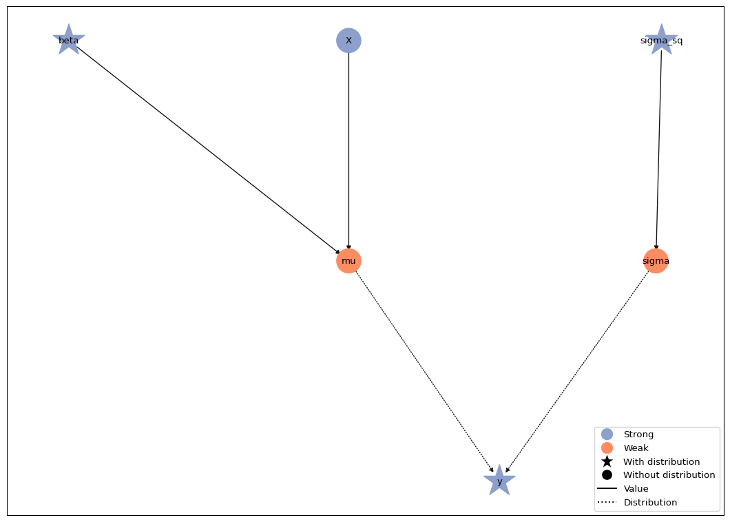
The plot_vars() function visualizes the model. More on that in the Model building with Liesel tutorial If the layout of the graph looks messy for you, please make sure you have the pygraphviz package installed.

lsl.plot_vars(model)

MCMC inference with Goose#

This section illustrates the basics of Liesel’s MCMC framework Goose. To use Goose, the user needs to select one or more sampling algorithms, called (transition) kernels, for the model parameters. Goose comes with a number of standard kernels such as Hamiltonian Monte Carlo (HMCKernel) or the No U-Turn Sampler (NUTSKernel). Multiple kernels can be combined in one sampling scheme and assigned to different parameters, and the user can implement their own problem-specific kernels, as long as they are compatible with the Kernel protocol. In any case, the user is responsible for constructing a mathematically valid algorithm.

We start with a very simple sampling scheme, keeping \(\sigma^2\) fixed at the true value and using a NUTS sampler for \(\boldsymbol{\beta}\). More on sampling \(\sigma^2\) can be found in the Parameter transformations tutorial and the Gibbs sampling tutorial. The kernels are added to a Engine, which coordinates the sampling, including the kernel tuning during the warmup, and the MCMC bookkeeping. The engine can be configured step by step with a EngineBuilder. Starting from a Liesel model, it is straight-forward to obtain an engine builder using the LieselMCMC helper. We then need to define the kernels, and the sampling duration. Finally, we can call the EngineBuilder.build() method, which returns a fully configured MCMC engine.

builder = gs.LieselMCMC(model).get_engine_builder(seed=1337, num_chains=4)

builder.add_kernel(gs.NUTSKernel(["beta"]))
builder.set_duration(warmup_duration=1000, posterior_duration=1000)

engine = builder.build()

Now we can run the MCMC algorithm for the specified duration by calling the sample_all_epochs() method. In a first step, the model and the sampling algorithm are compiled, so don’t worry if you don’t see an output right away. The subsequent samples will be generated much faster.

engine.sample_all_epochs()

  0%|                                                  | 0/3 [00:00<?, ?chunk/s]
 33%|##############                            | 1/3 [00:01<00:02,  1.35s/chunk]
100%|##########################################| 3/3 [00:01<00:00,  2.22chunk/s]

  0%|                                                  | 0/1 [00:00<?, ?chunk/s]
100%|########################################| 1/1 [00:00<00:00, 2212.19chunk/s]

  0%|                                                  | 0/2 [00:00<?, ?chunk/s]
100%|########################################| 2/2 [00:00<00:00, 3883.61chunk/s]

  0%|                                                  | 0/4 [00:00<?, ?chunk/s]
100%|########################################| 4/4 [00:00<00:00, 4106.02chunk/s]

  0%|                                                  | 0/8 [00:00<?, ?chunk/s]
100%|########################################| 8/8 [00:00<00:00, 1306.54chunk/s]

  0%|                                                 | 0/20 [00:00<?, ?chunk/s]
100%|#######################################| 20/20 [00:00<00:00, 391.76chunk/s]

  0%|                                                  | 0/2 [00:00<?, ?chunk/s]
100%|########################################| 2/2 [00:00<00:00, 2500.33chunk/s]

  0%|                                                 | 0/40 [00:00<?, ?chunk/s]
 82%|################################1      | 33/40 [00:00<00:00, 318.94chunk/s]
100%|#######################################| 40/40 [00:00<00:00, 303.65chunk/s]

Finally, we can extract the results and print a summary table.

results = engine.get_results()
summary = gs.Summary(results)
summary

Parameter summary:

		kernel	mean	sd	q_0.05	q_0.5	q_0.95	sample_size	ess_bulk	ess_tail	rhat
parameter	index
beta	(0,)	kernel_00	0.981	0.087	0.842	0.980	1.127	4000	887.081	1154.253	1.003
beta	(1,)	kernel_00	1.914	0.152	1.658	1.915	2.163	4000	883.961	1324.823	1.001

Error summary:

				count	sample_size	sample_size_total	relative
kernel	error_code	error_msg	phase
kernel_00	1	divergent transition	warmup	52	4000	4000	0.013
kernel_00	1	divergent transition	posterior	0	4000	4000	0.000

If we need more samples, we can append another epoch to the engine and sample it by calling either the sample_next_epoch() or the sample_all_epochs() method. The epochs are described by EpochConfig objects.

engine.append_epoch(
    gs.EpochConfig(gs.EpochType.POSTERIOR, duration=1000, thinning=1, optional=None)
)
engine.sample_next_epoch()

  0%|                                                 | 0/40 [00:00<?, ?chunk/s]
 80%|###############################2       | 32/40 [00:00<00:00, 311.91chunk/s]
100%|#######################################| 40/40 [00:00<00:00, 298.62chunk/s]

No compilation is required at this point, so this is pretty fast.

Here, we end this first tutorial. We have learned how to build a linear regression model and seen how we can use Kernels for drawing MCMC samples - that is quite a bit for the start. Now, have fun modelling with Liesel!

Linear Regression

Contents