GEV responses#
In this tutorial, we illustrate how to set up a distributional
regression model with the generalized extreme value distribution as a
response distribution. We configure the model in Python with
Liesel-GAM, using
liesel_gam.TermBuilder for linear terms and P-splines. See the
Liesel-GAM documentation and
examples for a
broader overview of the available term types.
We simulate data from a GEV model with three distributional parameters:
The location parameter (\(\mu\)) is a function of an intercept and a non-linear covariate effect.
The scale parameter (\(\sigma\)) is a function of an intercept and a linear effect and uses a log-link.
The shape or concentration parameter (\(\xi\)) is a function of an intercept and a linear effect.
import jax
import jax.numpy as jnp
import matplotlib.pyplot as plt
import numpy as np
import seaborn as sns
import tensorflow_probability.substrates.jax.distributions as tfd

import liesel.goose as gs
import liesel.model as lsl
import liesel_gam as gam

sns.set_theme(style="whitegrid")
key = jax.random.PRNGKey(13)
n = 500

key, key_x0, key_x1, key_x2, key_y = jax.random.split(key, 5)

x0 = jax.random.uniform(key_x0, (n,))
x1 = jax.random.uniform(key_x1, (n,))
x2 = jax.random.uniform(key_x2, (n,))

true_loc = jnp.sin(2 * jnp.pi * x0)
true_scale = jnp.exp(-1.0 + x1)
true_concentration = 0.1 + x2

y = tfd.GeneralizedExtremeValue(
    loc=true_loc,
    scale=true_scale,
    concentration=true_concentration,
).sample(seed=key_y)

data = pd.DataFrame({
    "y": np.asarray(y),
    "intercept": np.ones_like(y),
    "x0": np.asarray(x0),
    "x1": np.asarray(x1),
    "x2": np.asarray(x2),
    "true_loc": np.asarray(true_loc),
    "true_scale": np.asarray(true_scale),
    "true_concentration": np.asarray(true_concentration),
})
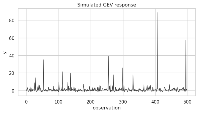
Here is the simulated response:
fig, ax = plt.subplots(figsize=(8, 4))
sns.lineplot(x=data.index, y=data["y"], ax=ax, color="0.25", linewidth=1)
ax.set(xlabel="observation", ylabel="y", title="Simulated GEV response")
plt.show()
We now construct the distributional regression model. The TermBuilder
reads the covariates from a pandas data frame and creates Liesel
variables for the corresponding model terms. The additive predictors are
passed directly to tfd.GeneralizedExtremeValue.
tb = gam.TermBuilder.from_df(data, default_inference=gs.MCMCSpec(gs.IWLSKernel))

loc = gam.AdditivePredictor("loc", intercept=True)
scale = gam.AdditivePredictor("scale", inv_link=jnp.exp, intercept=False)
concentration = gam.AdditivePredictor("concentration", intercept=False)

loc_smooth = tb.ps("x0", k=10)
scale_x1 = tb.lin("intercept + x1")
concentration_x2 = tb.lin("intercept + x2")

loc += loc_smooth
scale += scale_x1
concentration += concentration_x2

# The GEV distribution is numerically delicate around xi = 0, so we start away
# from the Gumbel case while keeping the linear effect initialized at zero.
concentration_x2.coef.value = jnp.array([0.1, 0.0])
concentration.update()

response_dist = lsl.Dist(
    tfd.GeneralizedExtremeValue,
    loc=loc,
    scale=scale,
    concentration=concentration,
)
y_var = lsl.Var.new_obs(data["y"].to_numpy(), response_dist, name="y")

model = lsl.Model([y_var])

# ScaleIG represents tau = sqrt(tau2). The Gibbs kernel samples tau2.
loc_smooth_tau2_name = loc_smooth.scale.value_node[0].name
We use Liesel’s MCMCSpec objects, which are added automatically by
Liesel-GAM, to set up the sampler. The default Liesel-GAM setup uses
IWLS kernels for regression coefficients and a Gibbs kernel for the
smoothing variance of the P-spline.
The support of the GEV distribution changes with the parameter values (compare Wikipedia).
results = gs.LieselMCMC(model).run_for_epochs(
    seed=1, num_chains=4, adaptation=1000, posterior=2500
)
gs.Summary(results)
liesel.goose.builder - WARNING - No jitter functions provided for position keys '$\\beta_{ps(x0)}$', '$\\tau_{ps(x0)}^2$', '$\\beta_{0,loc}$', '$\\beta_{lin(X)}$', '$\\beta_{lin(X1)}$'. The initial values for these keys won't be jittered
liesel.goose.engine - INFO - Initializing kernels...
liesel.goose.engine - INFO - Done
liesel.goose.engine - INFO - Starting epoch: FAST_ADAPTATION, 100 transitions, 25 jitted together

  0%|                                                  | 0/4 [00:00<?, ?chunk/s]
 25%|██████████▌                               | 1/4 [00:07<00:23,  8.00s/chunk]
100%|██████████████████████████████████████████| 4/4 [00:07<00:00,  2.00s/chunk]
liesel.goose.engine - WARNING - Errors per chain for kernel_00: 1, 1, 1, 1 / 100 transitions
liesel.goose.engine - WARNING - Errors per chain for kernel_03: 1, 1, 0, 2 / 100 transitions
liesel.goose.engine - WARNING - Errors per chain for kernel_04: 3, 2, 2, 3 / 100 transitions
liesel.goose.engine - INFO - Finished epoch
liesel.goose.engine - INFO - Starting epoch: SLOW_ADAPTATION, 25 transitions, 25 jitted together

  0%|                                                  | 0/1 [00:00<?, ?chunk/s]
100%|█████████████████████████████████████████| 1/1 [00:00<00:00, 655.56chunk/s]
liesel.goose.engine - WARNING - Errors per chain for kernel_00: 1, 2, 1, 1 / 25 transitions
liesel.goose.engine - WARNING - Errors per chain for kernel_03: 0, 1, 0, 1 / 25 transitions
liesel.goose.engine - WARNING - Errors per chain for kernel_04: 1, 2, 1, 1 / 25 transitions
liesel.goose.engine - INFO - Finished epoch
liesel.goose.engine - INFO - Starting epoch: SLOW_ADAPTATION, 50 transitions, 25 jitted together

  0%|                                                  | 0/2 [00:00<?, ?chunk/s]
100%|█████████████████████████████████████████| 2/2 [00:00<00:00, 869.56chunk/s]
liesel.goose.engine - WARNING - Errors per chain for kernel_00: 1, 1, 1, 0 / 50 transitions
liesel.goose.engine - WARNING - Errors per chain for kernel_03: 2, 0, 0, 2 / 50 transitions
liesel.goose.engine - WARNING - Errors per chain for kernel_04: 1, 3, 1, 2 / 50 transitions
liesel.goose.engine - INFO - Finished epoch
liesel.goose.engine - INFO - Starting epoch: SLOW_ADAPTATION, 100 transitions, 25 jitted together

  0%|                                                  | 0/4 [00:00<?, ?chunk/s]
100%|█████████████████████████████████████████| 4/4 [00:00<00:00, 833.11chunk/s]
liesel.goose.engine - WARNING - Errors per chain for kernel_00: 0, 1, 1, 1 / 100 transitions
liesel.goose.engine - WARNING - Errors per chain for kernel_03: 2, 0, 1, 2 / 100 transitions
liesel.goose.engine - WARNING - Errors per chain for kernel_04: 3, 1, 2, 1 / 100 transitions
liesel.goose.engine - INFO - Finished epoch
liesel.goose.engine - INFO - Starting epoch: SLOW_ADAPTATION, 525 transitions, 25 jitted together

  0%|                                                 | 0/21 [00:00<?, ?chunk/s]
 62%|████████████████████████▏              | 13/21 [00:00<00:00, 128.65chunk/s]
100%|████████████████████████████████████████| 21/21 [00:00<00:00, 91.13chunk/s]
liesel.goose.engine - WARNING - Errors per chain for kernel_00: 2, 3, 1, 2 / 525 transitions
liesel.goose.engine - WARNING - Errors per chain for kernel_03: 2, 3, 1, 1 / 525 transitions
liesel.goose.engine - WARNING - Errors per chain for kernel_04: 6, 5, 6, 4 / 525 transitions
liesel.goose.engine - INFO - Finished epoch
liesel.goose.engine - INFO - Starting epoch: FAST_ADAPTATION, 200 transitions, 25 jitted together

  0%|                                                  | 0/8 [00:00<?, ?chunk/s]
100%|█████████████████████████████████████████| 8/8 [00:00<00:00, 419.12chunk/s]
liesel.goose.engine - WARNING - Errors per chain for kernel_00: 2, 1, 1, 1 / 200 transitions
liesel.goose.engine - WARNING - Errors per chain for kernel_03: 2, 3, 3, 3 / 200 transitions
liesel.goose.engine - WARNING - Errors per chain for kernel_04: 4, 4, 3, 3 / 200 transitions
liesel.goose.engine - INFO - Finished epoch
liesel.goose.engine - INFO - Finished warmup
liesel.goose.engine - INFO - Starting epoch: POSTERIOR, 2500 transitions, 25 jitted together

  0%|                                                | 0/100 [00:00<?, ?chunk/s]
 13%|████▉                                 | 13/100 [00:00<00:00, 125.59chunk/s]
 26%|██████████▏                            | 26/100 [00:00<00:00, 78.75chunk/s]
 35%|█████████████▋                         | 35/100 [00:00<00:00, 71.65chunk/s]
 43%|████████████████▊                      | 43/100 [00:00<00:00, 68.22chunk/s]
 51%|███████████████████▉                   | 51/100 [00:00<00:00, 65.99chunk/s]
 58%|██████████████████████▌                | 58/100 [00:00<00:00, 64.71chunk/s]
 65%|█████████████████████████▎             | 65/100 [00:00<00:00, 63.85chunk/s]
 72%|████████████████████████████           | 72/100 [00:01<00:00, 63.27chunk/s]
 79%|██████████████████████████████▊        | 79/100 [00:01<00:00, 61.93chunk/s]
 86%|█████████████████████████████████▌     | 86/100 [00:01<00:00, 62.13chunk/s]
 93%|████████████████████████████████████▎  | 93/100 [00:01<00:00, 62.21chunk/s]
100%|██████████████████████████████████████| 100/100 [00:01<00:00, 62.33chunk/s]
100%|██████████████████████████████████████| 100/100 [00:01<00:00, 66.16chunk/s]
liesel.goose.engine - WARNING - Errors per chain for kernel_04: 4, 0, 0, 0 / 2500 transitions
liesel.goose.engine - INFO - Finished epoch
Parameter summary:
|
kernel |
mean |
sd |
q_0.05 |
q_0.5 |
q_0.95 |
sample_size |
ess_bulk |
ess_tail |
rhat |
||
|---|---|---|---|---|---|---|---|---|---|---|---|
|
parameter |
index |
||||||||||
|
\(\beta_{0,loc}\) |
() |
kernel_02 |
0.003 |
0.025 |
-0.037 |
0.002 |
0.045 |
10000 |
214.837 |
382.670 |
1.011 |
|
\(\beta_{lin(X)}\) |
(0,) |
kernel_03 |
-1.219 |
0.097 |
-1.376 |
-1.219 |
-1.059 |
10000 |
235.405 |
469.436 |
1.011 |
|
(1,) |
kernel_03 |
1.398 |
0.137 |
1.171 |
1.396 |
1.623 |
10000 |
347.217 |
718.748 |
1.006 |
|
|
\(\beta_{lin(X1)}\) |
(0,) |
kernel_04 |
0.104 |
0.095 |
-0.053 |
0.104 |
0.261 |
10000 |
393.226 |
657.114 |
1.029 |
|
(1,) |
kernel_04 |
1.016 |
0.186 |
0.714 |
1.014 |
1.324 |
10000 |
248.072 |
417.764 |
1.044 |
|
|
\(\beta_{ps(x0)}\) |
(0,) |
kernel_00 |
0.076 |
0.118 |
-0.115 |
0.077 |
0.264 |
10000 |
292.479 |
406.475 |
1.019 |
|
(1,) |
kernel_00 |
0.001 |
0.116 |
-0.195 |
0.004 |
0.183 |
10000 |
424.687 |
745.922 |
1.010 |
|
|
(2,) |
kernel_00 |
0.045 |
0.126 |
-0.164 |
0.046 |
0.249 |
10000 |
327.496 |
558.780 |
1.005 |
|
|
(3,) |
kernel_00 |
-0.009 |
0.106 |
-0.186 |
-0.007 |
0.159 |
10000 |
416.445 |
664.015 |
1.007 |
|
|
(4,) |
kernel_00 |
-0.147 |
0.102 |
-0.309 |
-0.149 |
0.022 |
10000 |
327.856 |
560.983 |
1.016 |
|
|
(5,) |
kernel_00 |
0.043 |
0.070 |
-0.072 |
0.042 |
0.156 |
10000 |
382.097 |
567.497 |
1.019 |
|
|
(6,) |
kernel_00 |
-0.358 |
0.048 |
-0.439 |
-0.357 |
-0.283 |
10000 |
327.511 |
546.265 |
1.017 |
|
|
(7,) |
kernel_00 |
-0.000 |
0.020 |
-0.034 |
-0.000 |
0.032 |
10000 |
389.357 |
519.426 |
1.009 |
|
|
(8,) |
kernel_00 |
-0.048 |
0.060 |
-0.142 |
-0.049 |
0.053 |
10000 |
325.519 |
570.110 |
1.019 |
|
|
\(\tau_{ps(x0)}^2\) |
() |
kernel_01 |
0.031 |
0.022 |
0.012 |
0.025 |
0.067 |
10000 |
1800.746 |
3162.994 |
1.002 |
Acceptance probabilities:
|
acceptance_probability |
position_moved |
|||
|---|---|---|---|---|
|
kernel |
positions |
phase |
||
|
kernel_00 |
\(\beta_{ps(x0)}\) |
posterior |
0.821 |
0.817 |
|
warmup |
0.794 |
0.795 |
||
|
kernel_01 |
\(\tau_{ps(x0)}^2\) |
posterior |
1.000 |
1.000 |
|
warmup |
1.000 |
1.000 |
||
|
kernel_02 |
\(\beta_{0,loc}\) |
posterior |
0.884 |
0.884 |
|
warmup |
0.888 |
0.887 |
||
|
kernel_03 |
\(\beta_{lin(X)}\) |
posterior |
0.858 |
0.857 |
|
warmup |
0.793 |
0.789 |
||
|
kernel_04 |
\(\beta_{lin(X1)}\) |
posterior |
0.868 |
0.865 |
|
warmup |
0.794 |
0.794 |
Error summary:
|
count |
sample_size |
sample_size_total |
relative |
|||||
|---|---|---|---|---|---|---|---|---|
|
kernel |
positions |
error_code |
error_msg |
phase |
||||
|
kernel_00 |
\(\beta_{ps(x0)}\) |
90 |
nan acceptance prob |
warmup |
28 |
4000 |
4000 |
0.007 |
|
posterior |
0 |
10000 |
10000 |
0.000 |
||||
|
kernel_03 |
\(\beta_{lin(X)}\) |
90 |
nan acceptance prob |
warmup |
33 |
4000 |
4000 |
0.008 |
|
posterior |
0 |
10000 |
10000 |
0.000 |
||||
|
kernel_04 |
\(\beta_{lin(X1)}\) |
2 |
indefinite information matrix (fallback to identity) |
warmup |
1 |
4000 |
4000 |
0.000 |
|
posterior |
1 |
10000 |
10000 |
0.000 |
||||
|
90 |
nan acceptance prob |
warmup |
62 |
4000 |
4000 |
0.015 |
||
|
posterior |
0 |
10000 |
10000 |
0.000 |
||||
|
92 |
indefinite information matrix (fallback to identity) + nan acceptance prob |
warmup |
1 |
4000 |
4000 |
0.000 |
||
|
posterior |
3 |
10000 |
10000 |
0.000 |
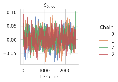
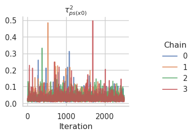
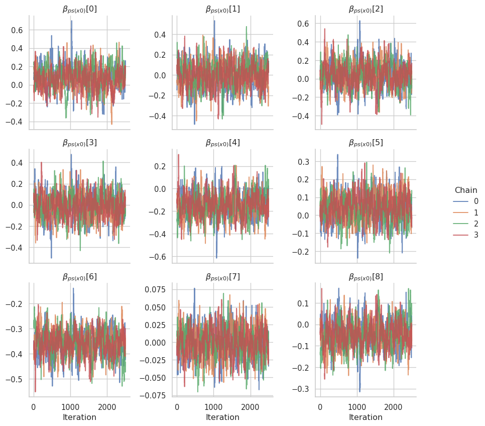
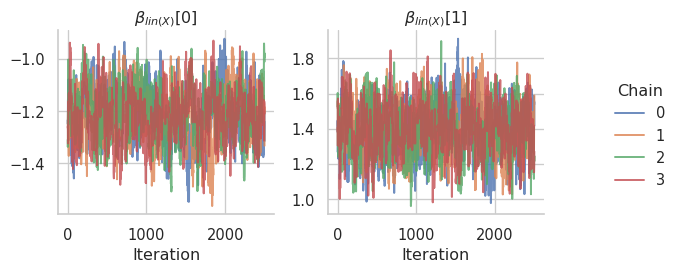
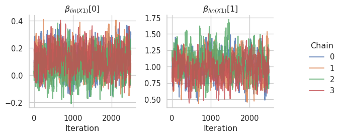
The corresponding trace plots:
gs.plot_trace(results, loc.intercept.name)
gs.plot_trace(results, loc_smooth_tau2_name)
gs.plot_trace(results, loc_smooth.coef.name)
gs.plot_trace(results, scale_x1.coef.name)
gs.plot_trace(results, concentration_x2.coef.name)
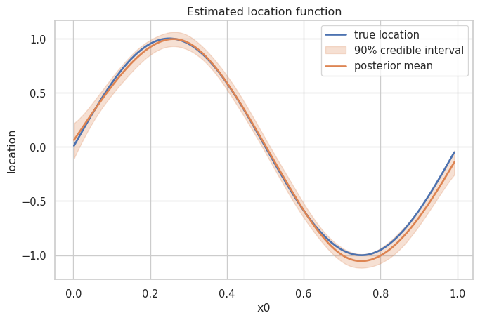
Finally, we can evaluate the posterior samples of the location predictor and compare the posterior mean with the true function used in the simulation.
samples = results.get_posterior_samples()
loc_samples = model.vars["loc"].predict(samples)
loc_summary = gs.SamplesSummary.from_array(
    loc_samples,
    name="loc",
    which=["mean", "quantiles"],
)
loc_summary_df = loc_summary.to_dataframe().reset_index()

loc_summary_df["x0"] = data["x0"].to_numpy()
loc_summary_df["true_loc"] = data["true_loc"].to_numpy()
loc_summary_df = loc_summary_df.sort_values("x0")

fig, ax = plt.subplots(figsize=(8, 5))
sns.lineplot(
    data=loc_summary_df,
    x="x0",
    y="true_loc",
    color=sns.color_palette()[0],
    linewidth=2,
    label="true location",
    ax=ax,
)
ax.fill_between(
    loc_summary_df["x0"],
    loc_summary_df["q_0.05"],
    loc_summary_df["q_0.95"],
    color=sns.color_palette()[1],
    alpha=0.25,
    label="90% credible interval",
)
sns.lineplot(
    data=loc_summary_df,
    x="x0",
    y="mean",
    color=sns.color_palette()[1],
    linewidth=2,
    label="posterior mean",
    ax=ax,
)

ax.set(xlabel="x0", ylabel="location", title="Estimated location function")
plt.show()