Comparing samplers#
In this tutorial, we compare two different sampling schemes on the
mcycle dataset with a Gaussian location-scale regression model and two
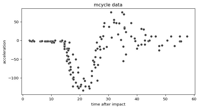
splines for the mean and the standard deviation. The mcycle dataset is
a “data frame giving a series of measurements of head acceleration in a
simulated motorcycle accident, used to test crash helmets” (from the
help page). It contains the following two variables:
times: in milliseconds after impactaccel: in g
We set up the model in Python with
Liesel-GAM, using
liesel_gam.TermBuilder for the P-spline terms. See the
Liesel-GAM documentation and
examples for more
information about additive terms and predictors. We load the data set
from R with ryp and then continue
with a pure Python model specification and sampling workflow.
from pathlib import Path

import jax.numpy as jnp
import matplotlib.pyplot as plt
import numpy as np
import seaborn as sns
import tensorflow_probability.substrates.jax.bijectors as tfb
import tensorflow_probability.substrates.jax.distributions as tfd

import liesel.goose as gs
import liesel.model as lsl
import liesel_gam as gam
from ryp import r, to_py
We start by loading the data set from the R package MASS and
converting it to a pandas data frame.
r("library(MASS)")
r("data(mcycle); mcycle <- as.data.frame(mcycle)")

mcycle = to_py("mcycle", format="pandas")
fig, ax = plt.subplots(figsize=(8, 4))
sns.scatterplot(data=mcycle, x="times", y="accel", color="0.25", s=35, ax=ax)
ax.set(xlabel="time after impact", ylabel="acceleration", title="mcycle data")
plt.show()
Next, we build the Gaussian location-scale model. Both distributional
parameters use an additive predictor with an intercept and a P-spline in
times. The scale predictor uses an exponential inverse link to keep
the standard deviation positive. The TermBuilder is initialized with
an IWLS MCMC specification, so the P-spline regression coefficients are
sampled with IWLS kernels by default. The additive predictor intercepts
also use their default IWLS inference specification. The smoothing
variances of the P-splines receive Gibbs kernels automatically.
tb = gam.TermBuilder.from_df(mcycle, default_inference=gs.MCMCSpec(gs.IWLSKernel))

loc = gam.AdditivePredictor("loc")
scale = gam.AdditivePredictor("scale", inv_link=jnp.exp)

loc_smooth = tb.ps("times", k=20, prefix="loc.")
scale_smooth = tb.ps("times", k=20, prefix="scale.")

loc += loc_smooth
scale += scale_smooth

response_dist = lsl.Dist(tfd.Normal, loc=loc, scale=scale)
y = lsl.Var.new_obs(mcycle["accel"], response_dist, name="y")
model = lsl.Model(y)
Metropolis-in-Gibbs#
First, we run the model with the inference specifications attached during model construction. This gives a Metropolis-in-Gibbs sampling scheme with IWLS kernels for the regression coefficients (\(\boldsymbol{\beta}\)) and Gibbs kernels for the smoothing variances (\(\tau^2\)) of the splines.
iwls_results = gs.LieselMCMC(model).run_for_epochs(
    seed=1, num_chains=4, adaptation=1000, posterior=10000, posterior_thinning=10, show_progress=False
)
liesel.goose.builder - WARNING - No jitter functions provided for position keys '$\\beta_{loc.ps(times)}$', '$\\beta_{scale.ps(times)}$', '$\\tau_{loc.ps(times)}^2$', '$\\beta_{0,loc}$', '$\\tau_{scale.ps(times)}^2$', '$\\beta_{0,scale}$'. The initial values for these keys won't be jittered
liesel.goose.engine - INFO - Initializing kernels...
liesel.goose.engine - INFO - Done
liesel.goose.engine - INFO - Finished warmup
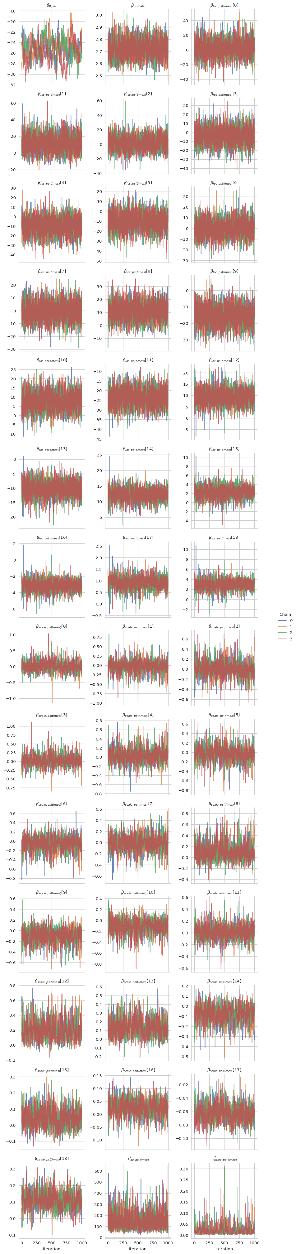
Clearly, the performance of the sampler could be better, especially for the intercept of the mean. The corresponding chain exhibits a very strong autocorrelation.
gs.Summary(iwls_results)
Parameter summary:
|
kernel |
mean |
sd |
q_0.05 |
q_0.5 |
q_0.95 |
sample_size |
ess_bulk |
ess_tail |
rhat |
||
|---|---|---|---|---|---|---|---|---|---|---|---|
|
parameter |
index |
||||||||||
|
\(\beta_{0,loc}\) |
() |
kernel_03 |
-25.231 |
1.982 |
-28.440 |
-25.266 |
-21.932 |
4000 |
91.735 |
99.749 |
1.043 |
|
\(\beta_{0,scale}\) |
() |
kernel_05 |
2.724 |
0.075 |
2.601 |
2.723 |
2.853 |
4000 |
1240.162 |
2309.053 |
1.002 |
|
\(\beta_{loc.ps(times)}\) |
(0,) |
kernel_00 |
2.389 |
10.804 |
-15.710 |
2.433 |
19.814 |
4000 |
2745.445 |
3217.044 |
1.000 |
|
(1,) |
kernel_00 |
11.079 |
10.199 |
-4.826 |
10.582 |
28.691 |
4000 |
2502.842 |
3212.205 |
1.000 |
|
|
(2,) |
kernel_00 |
1.566 |
9.327 |
-13.700 |
1.507 |
17.078 |
4000 |
2734.069 |
3514.793 |
1.000 |
|
|
(3,) |
kernel_00 |
-3.259 |
8.896 |
-18.092 |
-3.024 |
10.990 |
4000 |
3171.874 |
3456.306 |
1.001 |
|
|
(4,) |
kernel_00 |
-9.310 |
8.856 |
-24.442 |
-9.072 |
4.528 |
4000 |
3452.395 |
3637.538 |
1.001 |
|
|
(5,) |
kernel_00 |
-10.120 |
8.434 |
-24.343 |
-9.852 |
3.212 |
4000 |
2684.143 |
3569.892 |
1.001 |
|
|
(6,) |
kernel_00 |
0.110 |
7.682 |
-12.099 |
-0.028 |
12.989 |
4000 |
2973.361 |
2888.397 |
1.003 |
|
|
(7,) |
kernel_00 |
-0.425 |
7.055 |
-12.029 |
-0.529 |
11.258 |
4000 |
3317.425 |
3522.206 |
1.000 |
|
|
(8,) |
kernel_00 |
10.682 |
6.637 |
-0.434 |
10.657 |
21.660 |
4000 |
3410.736 |
3716.644 |
1.000 |
|
|
(9,) |
kernel_00 |
-15.615 |
5.729 |
-25.140 |
-15.519 |
-6.263 |
4000 |
2888.242 |
2849.860 |
1.001 |
|
|
(10,) |
kernel_00 |
7.597 |
4.886 |
-0.181 |
7.516 |
15.832 |
4000 |
2699.041 |
3273.765 |
1.001 |
|
|
(11,) |
kernel_00 |
-23.715 |
4.428 |
-31.150 |
-23.687 |
-16.500 |
4000 |
3119.502 |
3535.451 |
1.000 |
|
|
(12,) |
kernel_00 |
9.336 |
3.280 |
4.172 |
9.334 |
14.651 |
4000 |
3325.456 |
3589.285 |
1.001 |
|
|
(13,) |
kernel_00 |
-10.207 |
2.583 |
-14.431 |
-10.168 |
-6.068 |
4000 |
3216.028 |
3244.630 |
1.001 |
|
|
(14,) |
kernel_00 |
12.242 |
1.877 |
9.184 |
12.259 |
15.173 |
4000 |
3356.569 |
3364.785 |
1.001 |
|
|
(15,) |
kernel_00 |
2.242 |
1.235 |
0.189 |
2.249 |
4.188 |
4000 |
1827.116 |
2513.063 |
1.003 |
|
|
(16,) |
kernel_00 |
-3.139 |
0.646 |
-4.195 |
-3.124 |
-2.139 |
4000 |
3279.625 |
3283.467 |
1.001 |
|
|
(17,) |
kernel_00 |
0.912 |
0.242 |
0.524 |
0.919 |
1.291 |
4000 |
943.454 |
2046.986 |
1.004 |
|
|
(18,) |
kernel_00 |
2.983 |
0.925 |
1.523 |
3.007 |
4.375 |
4000 |
3234.198 |
2806.174 |
1.002 |
|
|
\(\beta_{scale.ps(times)}\) |
(0,) |
kernel_01 |
0.011 |
0.145 |
-0.213 |
0.005 |
0.256 |
4000 |
1157.099 |
1448.394 |
1.005 |
|
(1,) |
kernel_01 |
-0.024 |
0.149 |
-0.280 |
-0.016 |
0.198 |
4000 |
1200.021 |
1000.396 |
1.005 |
|
|
(2,) |
kernel_01 |
0.006 |
0.142 |
-0.215 |
0.002 |
0.238 |
4000 |
1351.423 |
1157.364 |
1.005 |
|
|
(3,) |
kernel_01 |
0.026 |
0.142 |
-0.194 |
0.022 |
0.264 |
4000 |
1183.395 |
1030.918 |
1.006 |
|
|
(4,) |
kernel_01 |
0.031 |
0.146 |
-0.191 |
0.022 |
0.284 |
4000 |
1099.421 |
722.438 |
1.007 |
|
|
(5,) |
kernel_01 |
-0.033 |
0.144 |
-0.272 |
-0.025 |
0.191 |
4000 |
1001.900 |
985.622 |
1.005 |
|
|
(6,) |
kernel_01 |
-0.056 |
0.145 |
-0.309 |
-0.043 |
0.159 |
4000 |
1086.999 |
1004.761 |
1.003 |
|
|
(7,) |
kernel_01 |
-0.017 |
0.133 |
-0.238 |
-0.015 |
0.196 |
4000 |
1058.990 |
1067.830 |
1.007 |
|
|
(8,) |
kernel_01 |
0.103 |
0.147 |
-0.100 |
0.080 |
0.374 |
4000 |
664.293 |
1027.972 |
1.011 |
|
|
(9,) |
kernel_01 |
-0.094 |
0.133 |
-0.324 |
-0.081 |
0.095 |
4000 |
870.111 |
1235.133 |
1.005 |
|
|
(10,) |
kernel_01 |
-0.116 |
0.120 |
-0.323 |
-0.108 |
0.059 |
4000 |
1030.726 |
1390.782 |
1.004 |
|
|
(11,) |
kernel_01 |
0.008 |
0.112 |
-0.169 |
0.011 |
0.185 |
4000 |
1044.794 |
1269.849 |
1.004 |
|
|
(12,) |
kernel_01 |
0.202 |
0.126 |
0.027 |
0.185 |
0.432 |
4000 |
435.379 |
606.760 |
1.011 |
|
|
(13,) |
kernel_01 |
0.138 |
0.099 |
-0.009 |
0.131 |
0.306 |
4000 |
625.898 |
1139.024 |
1.003 |
|
|
(14,) |
kernel_01 |
-0.079 |
0.085 |
-0.228 |
-0.072 |
0.046 |
4000 |
569.673 |
851.310 |
1.006 |
|
|
(15,) |
kernel_01 |
0.044 |
0.056 |
-0.039 |
0.039 |
0.138 |
4000 |
676.537 |
1207.682 |
1.005 |
|
|
(16,) |
kernel_01 |
0.026 |
0.032 |
-0.027 |
0.028 |
0.074 |
4000 |
582.852 |
778.132 |
1.014 |
|
|
(17,) |
kernel_01 |
-0.063 |
0.012 |
-0.081 |
-0.064 |
-0.042 |
4000 |
657.701 |
1249.209 |
1.007 |
|
|
(18,) |
kernel_01 |
0.111 |
0.048 |
0.033 |
0.111 |
0.191 |
4000 |
735.290 |
1102.061 |
1.013 |
|
|
\(\tau_{loc.ps(times)}^2\) |
() |
kernel_02 |
137.231 |
66.379 |
61.990 |
122.915 |
262.839 |
4000 |
2799.840 |
3249.357 |
1.000 |
|
\(\tau_{scale.ps(times)}^2\) |
() |
kernel_04 |
0.022 |
0.021 |
0.003 |
0.016 |
0.060 |
4000 |
303.019 |
492.178 |
1.021 |
Acceptance probabilities:
|
acceptance_probability |
position_moved |
|||
|---|---|---|---|---|
|
kernel |
positions |
phase |
||
|
kernel_00 |
\(\beta_{loc.ps(times)}\) |
posterior |
0.863 |
0.863 |
|
warmup |
0.794 |
0.793 |
||
|
kernel_01 |
\(\beta_{scale.ps(times)}\) |
posterior |
0.847 |
0.848 |
|
warmup |
0.793 |
0.790 |
||
|
kernel_02 |
\(\tau_{loc.ps(times)}^2\) |
posterior |
1.000 |
1.000 |
|
warmup |
1.000 |
1.000 |
||
|
kernel_03 |
\(\beta_{0,loc}\) |
posterior |
0.922 |
0.923 |
|
warmup |
0.923 |
0.927 |
||
|
kernel_04 |
\(\tau_{scale.ps(times)}^2\) |
posterior |
1.000 |
1.000 |
|
warmup |
1.000 |
1.000 |
||
|
kernel_05 |
\(\beta_{0,scale}\) |
posterior |
0.906 |
0.905 |
|
warmup |
0.912 |
0.909 |
gs.plot_trace(iwls_results)
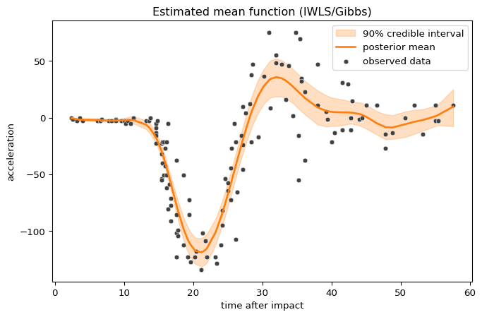
To confirm that the chains have converged to reasonable values, we plot the posterior mean of the location predictor together with a 90% credible interval:
def plot_loc_estimate(results, model, title):
    samples = results.get_posterior_samples()
    loc_samples = model.vars["loc"].predict(samples)
    loc_summary = gs.SamplesSummary.from_array(
        loc_samples,
        name="loc",
        which=["mean", "quantiles"],
    )
    loc_summary_df = loc_summary.to_dataframe().reset_index()

    loc_summary_df["times"] = mcycle["times"].to_numpy()
    plot_data = (
        loc_summary_df[["times", "mean", "q_0.05", "q_0.95"]]
        .groupby("times", as_index=False)
        .mean()
        .sort_values("times")
    )

    fig, ax = plt.subplots(figsize=(8, 5))
    ax.fill_between(
        plot_data["times"],
        plot_data["q_0.05"],
        plot_data["q_0.95"],
        color=sns.color_palette()[1],
        alpha=0.25,
        label="90% credible interval",
    )
    sns.lineplot(
        data=plot_data,
        x="times",
        y="mean",
        color=sns.color_palette()[1],
        linewidth=2,
        label="posterior mean",
        ax=ax,
    )
    sns.scatterplot(
        data=mcycle,
        x="times",
        y="accel",
        color="0.25",
        s=25,
        ax=ax,
        label="observed data",
    )
    ax.set(xlabel="time after impact", ylabel="acceleration", title=title)
    plt.show()


plot_loc_estimate(iwls_results, model, "Estimated mean function (IWLS/Gibbs)")
NUTS sampler#
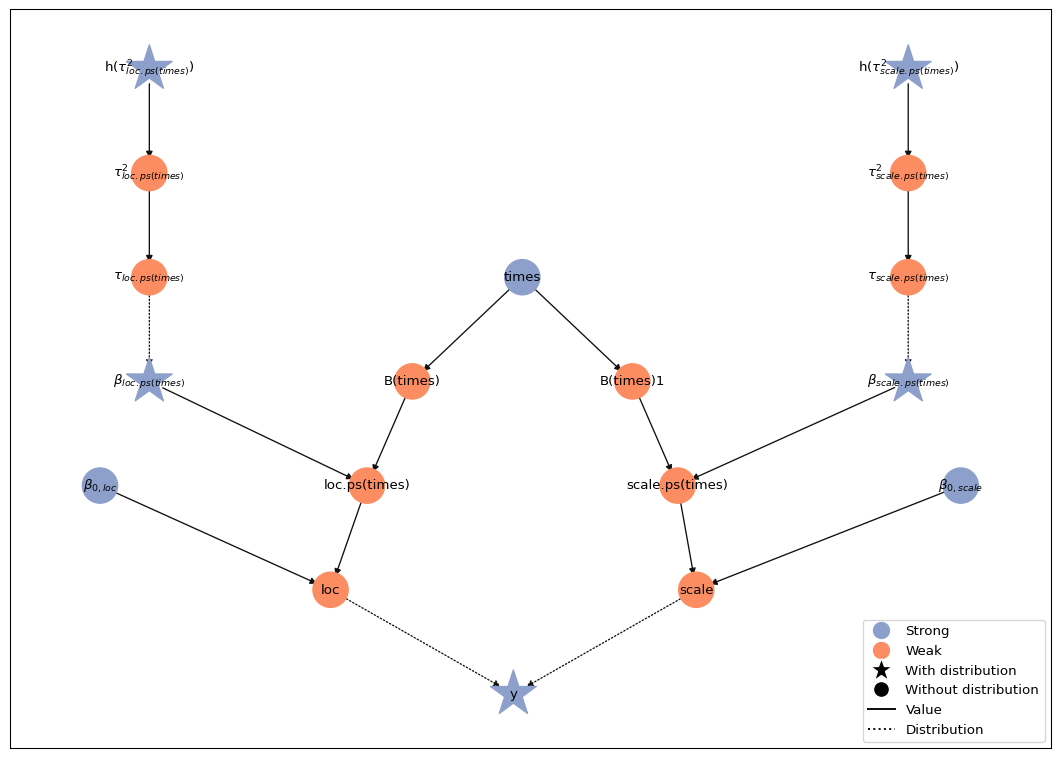
As an alternative, we use NUTS kernels for the spline-specific parameter blocks. The helper below copies the model graph, log-transforms the smoothing variances by bijecting them with an exponential bijector, and assigns one NUTS kernel group per additive term.
def strategy_term_blocked(
    model: lsl.Model, predictors: list[str], kernel_constructor, **kwargs
):
    model = model.copy()
    for k, v in model.parameters.items():
        if "tau" in k:
            v.biject(tfb.Exp(), inference="drop")

    for predictor_name in predictors:
        predictor = model.vars[predictor_name]
        if predictor.intercept:
            predictor.intercept.inference = gs.MCMCSpec(
                kernel_constructor, kernel_kwargs=kwargs
            )

        for term in predictor.terms.values():
            for param in model.parental_submodel(term).parameters.values():
                model.parameters[param.name].inference = gs.MCMCSpec(
                    kernel_constructor, kernel_group=term.name, kernel_kwargs=kwargs
                )

    return model
nuts_model = strategy_term_blocked(model, ["loc", "scale"], gs.NUTSKernel)
The resulting model contains transformed smoothing variances on the unconstrained log scale. Here is the transformed model graph:
nuts_model.plot()
Now we can run the sampler from the MCMCSpec objects stored in the
model. In complex models like this one, it can be beneficial to sample
the parameters of each additive term in a separate NUTS block.
nuts_results = gs.LieselMCMC(nuts_model).run_for_epochs(
    seed=1, num_chains=4, adaptation=1000, posterior=1000, show_progress=False
)
liesel.goose.builder - WARNING - No jitter functions provided for position keys '$\\beta_{loc.ps(times)}$', 'h($\\tau_{loc.ps(times)}^2$)', '$\\beta_{scale.ps(times)}$', 'h($\\tau_{scale.ps(times)}^2$)', '$\\beta_{0,loc}$', '$\\beta_{0,scale}$'. The initial values for these keys won't be jittered
liesel.goose.engine - INFO - Initializing kernels...
liesel.goose.engine - INFO - Done
liesel.goose.engine - INFO - Finished warmup
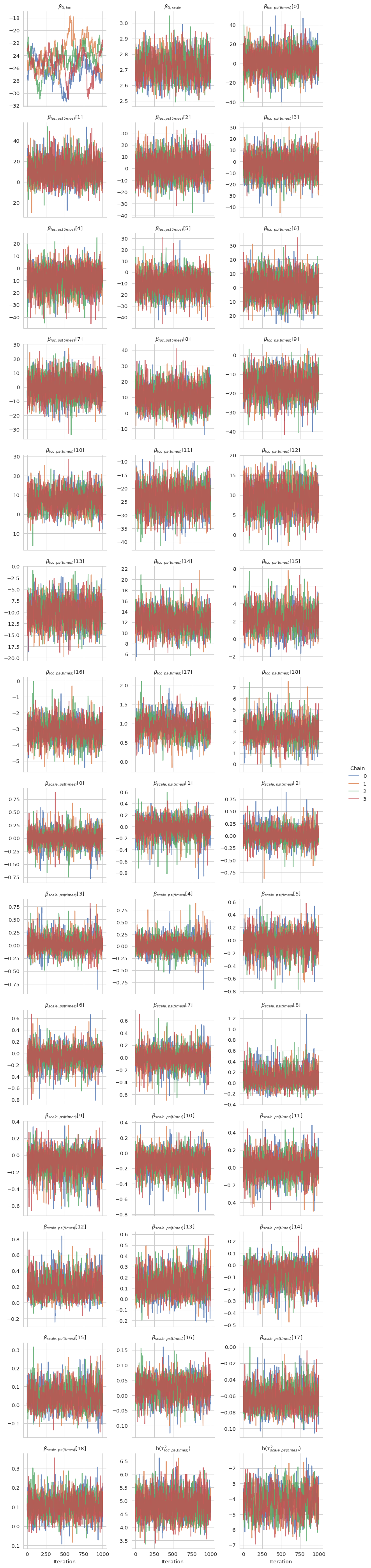
The blocked NUTS strategy overall seems to do a good job and can yield higher effective sample sizes than the IWLS sampler, especially for the spline coefficients of the scale model.
gs.Summary(nuts_results)
Parameter summary:
|
kernel |
mean |
sd |
q_0.05 |
q_0.5 |
q_0.95 |
sample_size |
ess_bulk |
ess_tail |
rhat |
||
|---|---|---|---|---|---|---|---|---|---|---|---|
|
parameter |
index |
||||||||||
|
\(\beta_{0,loc}\) |
() |
kernel_02 |
-25.157 |
2.255 |
-29.277 |
-25.095 |
-21.618 |
4000 |
13.116 |
15.298 |
1.240 |
|
\(\beta_{0,scale}\) |
() |
kernel_03 |
2.723 |
0.076 |
2.603 |
2.720 |
2.851 |
4000 |
675.615 |
1260.077 |
1.004 |
|
\(\beta_{loc.ps(times)}\) |
(0,) |
kernel_00 |
2.682 |
10.627 |
-14.695 |
2.687 |
19.847 |
4000 |
4064.084 |
2753.618 |
1.001 |
|
(1,) |
kernel_00 |
11.372 |
10.339 |
-4.712 |
10.733 |
29.440 |
4000 |
2718.144 |
2039.869 |
1.003 |
|
|
(2,) |
kernel_00 |
1.461 |
9.325 |
-14.031 |
1.412 |
16.753 |
4000 |
3319.317 |
2426.635 |
1.002 |
|
|
(3,) |
kernel_00 |
-3.353 |
8.916 |
-17.948 |
-3.249 |
11.335 |
4000 |
3185.618 |
2749.068 |
1.002 |
|
|
(4,) |
kernel_00 |
-9.362 |
8.880 |
-24.667 |
-9.085 |
4.699 |
4000 |
3058.779 |
2325.766 |
1.001 |
|
|
(5,) |
kernel_00 |
-10.313 |
8.543 |
-24.531 |
-10.120 |
3.330 |
4000 |
2856.079 |
2586.780 |
1.001 |
|
|
(6,) |
kernel_00 |
0.566 |
7.934 |
-12.275 |
0.369 |
13.514 |
4000 |
2530.758 |
2844.444 |
1.002 |
|
|
(7,) |
kernel_00 |
-0.235 |
7.445 |
-12.426 |
-0.319 |
12.225 |
4000 |
2481.104 |
2443.635 |
1.001 |
|
|
(8,) |
kernel_00 |
10.731 |
6.754 |
-0.296 |
10.691 |
22.074 |
4000 |
2269.861 |
2242.519 |
1.002 |
|
|
(9,) |
kernel_00 |
-15.589 |
5.883 |
-25.395 |
-15.445 |
-6.031 |
4000 |
1590.324 |
2105.093 |
1.003 |
|
|
(10,) |
kernel_00 |
7.504 |
4.913 |
-0.469 |
7.489 |
15.721 |
4000 |
1014.294 |
1676.991 |
1.004 |
|
|
(11,) |
kernel_00 |
-23.858 |
4.530 |
-31.420 |
-23.791 |
-16.633 |
4000 |
1352.847 |
1894.121 |
1.002 |
|
|
(12,) |
kernel_00 |
9.164 |
3.213 |
3.938 |
9.161 |
14.466 |
4000 |
1170.496 |
1725.139 |
1.006 |
|
|
(13,) |
kernel_00 |
-10.156 |
2.535 |
-14.347 |
-10.178 |
-6.043 |
4000 |
1191.233 |
1847.846 |
1.005 |
|
|
(14,) |
kernel_00 |
12.291 |
1.875 |
9.226 |
12.301 |
15.349 |
4000 |
1192.178 |
1541.098 |
1.004 |
|
|
(15,) |
kernel_00 |
2.294 |
1.234 |
0.292 |
2.276 |
4.301 |
4000 |
522.760 |
1089.537 |
1.012 |
|
|
(16,) |
kernel_00 |
-3.120 |
0.627 |
-4.142 |
-3.120 |
-2.098 |
4000 |
989.886 |
1481.136 |
1.005 |
|
|
(17,) |
kernel_00 |
0.914 |
0.246 |
0.510 |
0.917 |
1.307 |
4000 |
96.340 |
863.558 |
1.037 |
|
|
(18,) |
kernel_00 |
3.011 |
0.907 |
1.557 |
3.008 |
4.498 |
4000 |
928.757 |
1363.198 |
1.004 |
|
|
\(\beta_{scale.ps(times)}\) |
(0,) |
kernel_01 |
0.001 |
0.141 |
-0.219 |
0.001 |
0.217 |
4000 |
4692.991 |
1962.539 |
1.002 |
|
(1,) |
kernel_01 |
-0.024 |
0.143 |
-0.273 |
-0.016 |
0.192 |
4000 |
4934.493 |
1801.269 |
1.003 |
|
|
(2,) |
kernel_01 |
0.011 |
0.146 |
-0.211 |
0.007 |
0.251 |
4000 |
5073.525 |
1989.663 |
1.005 |
|
|
(3,) |
kernel_01 |
0.029 |
0.142 |
-0.186 |
0.022 |
0.264 |
4000 |
4361.999 |
1997.520 |
1.001 |
|
|
(4,) |
kernel_01 |
0.026 |
0.144 |
-0.192 |
0.020 |
0.257 |
4000 |
4809.598 |
1909.172 |
1.003 |
|
|
(5,) |
kernel_01 |
-0.032 |
0.144 |
-0.281 |
-0.026 |
0.188 |
4000 |
5427.737 |
1621.686 |
1.003 |
|
|
(6,) |
kernel_01 |
-0.056 |
0.143 |
-0.302 |
-0.046 |
0.156 |
4000 |
3333.762 |
1551.118 |
1.000 |
|
|
(7,) |
kernel_01 |
-0.012 |
0.132 |
-0.225 |
-0.009 |
0.196 |
4000 |
4524.246 |
2200.880 |
1.003 |
|
|
(8,) |
kernel_01 |
0.093 |
0.145 |
-0.109 |
0.075 |
0.361 |
4000 |
1907.307 |
1375.404 |
1.002 |
|
|
(9,) |
kernel_01 |
-0.090 |
0.125 |
-0.308 |
-0.076 |
0.090 |
4000 |
2468.683 |
2047.995 |
1.003 |
|
|
(10,) |
kernel_01 |
-0.120 |
0.122 |
-0.337 |
-0.107 |
0.057 |
4000 |
2564.739 |
2204.354 |
1.002 |
|
|
(11,) |
kernel_01 |
0.009 |
0.114 |
-0.181 |
0.009 |
0.195 |
4000 |
3307.058 |
2243.883 |
1.002 |
|
|
(12,) |
kernel_01 |
0.204 |
0.122 |
0.028 |
0.193 |
0.421 |
4000 |
814.724 |
1340.109 |
1.003 |
|
|
(13,) |
kernel_01 |
0.138 |
0.100 |
-0.009 |
0.133 |
0.309 |
4000 |
1246.340 |
1565.672 |
1.002 |
|
|
(14,) |
kernel_01 |
-0.083 |
0.085 |
-0.231 |
-0.078 |
0.043 |
4000 |
971.161 |
1790.243 |
1.002 |
|
|
(15,) |
kernel_01 |
0.044 |
0.058 |
-0.044 |
0.040 |
0.145 |
4000 |
1184.525 |
1425.558 |
1.004 |
|
|
(16,) |
kernel_01 |
0.024 |
0.033 |
-0.033 |
0.026 |
0.074 |
4000 |
1052.191 |
1817.478 |
1.004 |
|
|
(17,) |
kernel_01 |
-0.063 |
0.013 |
-0.083 |
-0.063 |
-0.040 |
4000 |
1309.675 |
1534.598 |
1.001 |
|
|
(18,) |
kernel_01 |
0.108 |
0.049 |
0.026 |
0.109 |
0.187 |
4000 |
1391.988 |
1917.419 |
1.004 |
|
|
h(\(\tau_{loc.ps(times)}^2\)) |
() |
kernel_00 |
4.835 |
0.440 |
4.135 |
4.827 |
5.593 |
4000 |
1654.489 |
1923.113 |
1.001 |
|
h(\(\tau_{scale.ps(times)}^2\)) |
() |
kernel_01 |
-4.184 |
0.841 |
-5.620 |
-4.138 |
-2.859 |
4000 |
363.985 |
693.435 |
1.006 |
Acceptance probabilities:
|
acceptance_probability |
position_moved |
|||
|---|---|---|---|---|
|
kernel |
positions |
phase |
||
|
kernel_00 |
\(\beta_{loc.ps(times)}\), h(\(\tau_{loc.ps(times)}^2\)) |
posterior |
0.892 |
NaN |
|
warmup |
0.793 |
NaN |
||
|
kernel_01 |
\(\beta_{scale.ps(times)}\), h(\(\tau_{scale.ps(times)}^2\)) |
posterior |
0.876 |
NaN |
|
warmup |
0.794 |
NaN |
||
|
kernel_02 |
\(\beta_{0,loc}\) |
posterior |
0.862 |
NaN |
|
warmup |
0.791 |
NaN |
||
|
kernel_03 |
\(\beta_{0,scale}\) |
posterior |
0.875 |
NaN |
|
warmup |
0.793 |
NaN |
Error summary:
|
count |
sample_size |
sample_size_total |
relative |
|||||
|---|---|---|---|---|---|---|---|---|
|
kernel |
positions |
error_code |
error_msg |
phase |
||||
|
kernel_00 |
\(\beta_{loc.ps(times)}\), h(\(\tau_{loc.ps(times)}^2\)) |
1 |
divergent transition |
warmup |
364 |
4000 |
4000 |
0.091 |
|
posterior |
18 |
4000 |
4000 |
0.004 |
||||
|
2 |
maximum tree depth |
warmup |
393 |
4000 |
4000 |
0.098 |
||
|
posterior |
0 |
4000 |
4000 |
0.000 |
||||
|
kernel_01 |
\(\beta_{scale.ps(times)}\), h(\(\tau_{scale.ps(times)}^2\)) |
1 |
divergent transition |
warmup |
272 |
4000 |
4000 |
0.068 |
|
posterior |
0 |
4000 |
4000 |
0.000 |
||||
|
2 |
maximum tree depth |
warmup |
8 |
4000 |
4000 |
0.002 |
||
|
posterior |
0 |
4000 |
4000 |
0.000 |
||||
|
kernel_02 |
\(\beta_{0,loc}\) |
1 |
divergent transition |
warmup |
75 |
4000 |
4000 |
0.019 |
|
posterior |
0 |
4000 |
4000 |
0.000 |
||||
|
kernel_03 |
\(\beta_{0,scale}\) |
1 |
divergent transition |
warmup |
36 |
4000 |
4000 |
0.009 |
|
posterior |
0 |
4000 |
4000 |
0.000 |
gs.plot_trace(nuts_results)
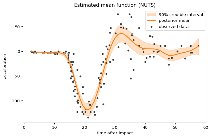
Again, here is the posterior mean function with a 90% credible interval:
plot_loc_estimate(nuts_results, nuts_model, "Estimated mean function (NUTS)")