Gibbs Sampling#
This tutorial extends the linear regression tutorial. Here, we show how to sample model parameters using a Gibbs kernel.
As this tutorial is a continuation of the previous tutorials, we will use the same model and data assumed there.
Data and imports#
import jax
import jax.numpy as jnp
import numpy as np

# We use distributions and bijectors from tensorflow probability
import tensorflow_probability.substrates.jax.distributions as tfd
import tensorflow_probability.substrates.jax.bijectors as tfb

import liesel.goose as gs
import liesel.model as lsl

import matplotlib.pyplot as plt
# Generate data
rng = np.random.default_rng(42)

# sample size and true parameters
n = 500
true_beta = np.array([1.0, 2.0])
true_sigma = 1.0

# data-generating process
x0 = rng.uniform(size=n)
X_mat = np.column_stack([np.ones(n), x0])
eps = rng.normal(scale=true_sigma, size=n)
y_vec = X_mat @ true_beta + eps

# define beta
beta_prior = lsl.Dist(tfd.Normal, loc=0.0, scale=100.0)

beta = lsl.Var.new_param(value=jnp.array([0.0, 0.0]), dist=beta_prior, name="beta")

# define the variance and the scale
a = lsl.Var.new_param(0.01, name="a")
b = lsl.Var.new_param(0.01, name="b")
sigma_sq_prior = lsl.Dist(tfd.InverseGamma, concentration=a, scale=b)
sigma_sq = lsl.Var.new_param(value=1.0, dist=sigma_sq_prior, name="sigma_sq")

# Define sigma as a transformation of sigma_sq for the likelihood
sigma = lsl.Var.new_calc(jnp.sqrt, sigma_sq, name="sigma")

# calculator-setup
X = lsl.Var.new_obs(X_mat, name="X")
mu = lsl.Var.new_calc(jnp.dot, X, beta, name="mu")

# Build response
y_dist = lsl.Dist(tfd.Normal, loc=mu, scale=sigma)
y = lsl.Var.new_obs(y_vec, dist=y_dist, name="y")

# Plot model
model = lsl.Model([y])
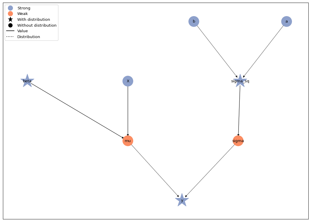
model.plot()
MCMC inference#
Using a Gibbs kernel#
This time we want to sample the previously fixed sigma_sq with a Gibbs
sampler. Using a Gibbs kernel is a bit more complicated, because Goose
doesn’t automatically derive the full conditional from the model graph.
Hence, the user needs to provide a function to sample from the full
conditional. The function needs to accept a PRNG key and a model state
as arguments, and it needs to return a dictionary with the variable name
as the key and the new variable value as the value. We could also update
multiple parameters with one Gibbs kernel by returning a dictionary with
several entries.
For this normal-inverse-gamma model, the full conditional of \(\sigma^2\)
is again an inverse-gamma distribution. To retrieve the relevant values
from the model_state, we use Model.extract_position().
def draw_sigma_sq(prng_key, model_state):
    # extract relevant values from model state
    pos = model.extract_position(
        position_keys=["y", "mu", "sigma_sq", "a", "b"], model_state=model_state
    )
    # calculate relevant intermediate quantities
    n = len(pos["y"])
    resid = pos["y"] - pos["mu"]
    a_gibbs = pos["a"] + n / 2
    b_gibbs = pos["b"] + jnp.sum(resid**2) / 2
    # draw new value from full conditional
    draw = b_gibbs / jax.random.gamma(prng_key, a_gibbs)
    # return key-value pair of variable name and new value
    return {"sigma_sq": draw}
The regression coefficients beta are still sampled with NUTS. For
sigma_sq, we attach an MCMCSpec with
with_transition_fn(), which turns our custom
transition function into a kernel factory that LieselMCMC can
use. The Gibbs kernel itself does not need adaptation, but the NUTS
kernel for beta does, so we still run an adaptation phase before
drawing posterior samples.
beta.inference = gs.MCMCSpec(gs.NUTSKernel)
sigma_sq.inference = gs.MCMCSpec(gs.GibbsKernel.with_transition_fn(draw_sigma_sq))

results = gs.LieselMCMC(model).run_for_epochs(
    seed=1, num_chains=4, adaptation=1000, posterior=1000
)
liesel.goose.mcmc_spec - WARNING - No inference specification defined for Var(name="b"). If you do not add a kernel for this parameter manually to an EngineBuilder, it will not be sampled.
liesel.goose.mcmc_spec - WARNING - No inference specification defined for Var(name="a"). If you do not add a kernel for this parameter manually to an EngineBuilder, it will not be sampled.
liesel.goose.builder - WARNING - No jitter functions provided for position keys 'sigma_sq', 'beta'. The initial values for these keys won't be jittered
liesel.goose.engine - INFO - Initializing kernels...
liesel.goose.engine - INFO - Done
liesel.goose.engine - INFO - Starting epoch: FAST_ADAPTATION, 100 transitions, 25 jitted together

  0%|                                                  | 0/4 [00:00<?, ?chunk/s]
 25%|██████████▌                               | 1/4 [00:03<00:10,  3.49s/chunk]
100%|██████████████████████████████████████████| 4/4 [00:03<00:00,  1.14chunk/s]
liesel.goose.engine - WARNING - Errors per chain for kernel_01: 2, 4, 4, 2 / 100 transitions
liesel.goose.engine - INFO - Finished epoch
liesel.goose.engine - INFO - Starting epoch: SLOW_ADAPTATION, 25 transitions, 25 jitted together

  0%|                                                  | 0/1 [00:00<?, ?chunk/s]
100%|████████████████████████████████████████| 1/1 [00:00<00:00, 1007.76chunk/s]
liesel.goose.engine - WARNING - Errors per chain for kernel_01: 1, 2, 1, 1 / 25 transitions
liesel.goose.engine - INFO - Finished epoch
liesel.goose.engine - INFO - Starting epoch: SLOW_ADAPTATION, 50 transitions, 25 jitted together

  0%|                                                  | 0/2 [00:00<?, ?chunk/s]
100%|████████████████████████████████████████| 2/2 [00:00<00:00, 1002.34chunk/s]
liesel.goose.engine - WARNING - Errors per chain for kernel_01: 1, 3, 1, 1 / 50 transitions
liesel.goose.engine - INFO - Finished epoch
liesel.goose.engine - INFO - Starting epoch: SLOW_ADAPTATION, 100 transitions, 25 jitted together

  0%|                                                  | 0/4 [00:00<?, ?chunk/s]
100%|████████████████████████████████████████| 4/4 [00:00<00:00, 1659.96chunk/s]
liesel.goose.engine - WARNING - Errors per chain for kernel_01: 1, 2, 1, 1 / 100 transitions
liesel.goose.engine - INFO - Finished epoch
liesel.goose.engine - INFO - Starting epoch: SLOW_ADAPTATION, 525 transitions, 25 jitted together

  0%|                                                 | 0/21 [00:00<?, ?chunk/s]
100%|███████████████████████████████████████| 21/21 [00:00<00:00, 298.33chunk/s]
liesel.goose.engine - WARNING - Errors per chain for kernel_01: 4, 3, 2, 3 / 525 transitions
liesel.goose.engine - INFO - Finished epoch
liesel.goose.engine - INFO - Starting epoch: FAST_ADAPTATION, 200 transitions, 25 jitted together

  0%|                                                  | 0/8 [00:00<?, ?chunk/s]
100%|████████████████████████████████████████| 8/8 [00:00<00:00, 1142.08chunk/s]
liesel.goose.engine - WARNING - Errors per chain for kernel_01: 3, 1, 2, 4 / 200 transitions
liesel.goose.engine - INFO - Finished epoch
liesel.goose.engine - INFO - Finished warmup
liesel.goose.engine - INFO - Starting epoch: POSTERIOR, 1000 transitions, 25 jitted together

  0%|                                                 | 0/40 [00:00<?, ?chunk/s]
 75%|█████████████████████████████▎         | 30/40 [00:00<00:00, 293.62chunk/s]
100%|███████████████████████████████████████| 40/40 [00:00<00:00, 274.01chunk/s]
liesel.goose.engine - INFO - Finished epoch
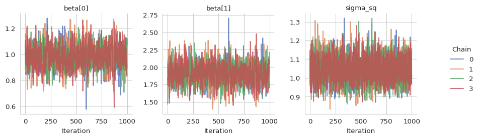
Finally, we can take a look at our results.
summary = gs.Summary(results)
summary
Parameter summary:
|
kernel |
mean |
sd |
q_0.05 |
q_0.5 |
q_0.95 |
sample_size |
ess_bulk |
ess_tail |
rhat |
||
|---|---|---|---|---|---|---|---|---|---|---|---|
|
parameter |
index |
||||||||||
|
beta |
(0,) |
kernel_01 |
0.983 |
0.090 |
0.837 |
0.984 |
1.128 |
4000 |
946.958 |
1138.096 |
1.007 |
|
(1,) |
kernel_01 |
1.912 |
0.154 |
1.661 |
1.913 |
2.158 |
4000 |
933.683 |
1052.928 |
1.007 |
|
|
sigma_sq |
() |
kernel_00 |
1.043 |
0.066 |
0.939 |
1.040 |
1.154 |
4000 |
4091.178 |
3815.673 |
1.000 |
Acceptance probabilities:
|
acceptance_probability |
position_moved |
|||
|---|---|---|---|---|
|
kernel |
positions |
phase |
||
|
kernel_00 |
sigma_sq |
posterior |
1.000 |
1.000 |
|
warmup |
1.000 |
1.000 |
||
|
kernel_01 |
beta |
posterior |
0.885 |
NaN |
|
warmup |
0.791 |
NaN |
Error summary:
|
count |
sample_size |
sample_size_total |
relative |
|||||
|---|---|---|---|---|---|---|---|---|
|
kernel |
positions |
error_code |
error_msg |
phase |
||||
|
kernel_01 |
beta |
1 |
divergent transition |
warmup |
50 |
4000 |
4000 |
0.012 |
|
posterior |
0 |
4000 |
4000 |
0.000 |
And plot them.
gs.plot_trace(results)