Monitor a fit

loss_monitor chooses the loss used for early stopping and for saving the best fit. Choose it when creating liesel.optim.LieselOptim.

Setting	Use it when	What is measured
"validation"	You have held-out validation data.	Full validation loss after each epoch.
"train_full_data"	You want to check the full training objective.	Full training loss after each epoch.
opt.EmaTrainLossMonitor(effective_window=2.0)	Full-data checks are too expensive.	A running average of minibatch training losses.

An epoch runs all configured batches. The two full-data monitors each add one loss evaluation at the end of every epoch. Validation uses likelihood only by default; set validation_strategy="log_prob" to include priors.

This page uses a small Gaussian regression. Expand the setup to run the examples from top to bottom.

import logging

import jax.numpy as jnp
import numpy as np
import optax
import tensorflow_probability.substrates.jax.distributions as tfd

import liesel.model as lsl
import liesel.optim as opt

Show code cell source

Hide code cell source

logging.getLogger("liesel").setLevel(logging.WARNING)

rng = np.random.default_rng(42)
x = np.linspace(-1.0, 1.0, 128)
X = lsl.Var.new_obs(jnp.asarray(x), name="X")
beta = lsl.Var.new_param(0.0, lsl.Dist(tfd.Normal, 0.0, 5.0), name="beta")
log_sigma = lsl.Var.new_param(0.0, name="log_sigma")
sigma = lsl.Var.new_calc(jnp.exp, log_sigma, name="sigma")
mu = lsl.Var.new_calc(lambda X, beta: X * beta, X, beta, name="mu")
y = lsl.Var.new_obs(
    jnp.asarray(0.5 * x + rng.normal(scale=0.7, size=x.size)),
    lsl.Dist(tfd.Normal, mu, sigma),
    name="y",
)
model = lsl.Model(y)

Choose when to stop

stopper = opt.Stopper(epochs=500, patience=20, rtol=1e-4)
builder = opt.LieselOptim(
    model,
    optimizers=optax.adam(0.01),
    loss_monitor="train_full_data",
    stopper=stopper,
    show_progress=False,
)
result = builder.fit()

This allows at most 500 epochs. Within the last 20 epochs, fitting stops when there is no worthwhile improvement over the oldest loss in that window. atol measures absolute improvement; rtol measures relative improvement. See Stopper for the exact rule.

Read the result

result.status

'early_stopping'

result.position_min_monitor

{'beta': Array(0.43896037, dtype=float32, weak_type=True),
 'log_sigma': Array(-0.5868051, dtype=float32, weak_type=True)}

• result.position_min_monitor holds the parameters saved at the epoch with the lowest finite monitoring loss. It raises RuntimeError if no such loss was recorded. An earlier best position remains available after a later failure.

• result.position_final holds the parameters at the end of the run.

• result.plot_loss_overview() shows the full loss history and a closer view of recent epochs.

• result.plot_params() shows saved parameter paths.

Both position properties raise RuntimeError if their parameters contain NaN or infinity. History, status, and diagnostics remain available for inspection. See Investigate NaNs to capture information about a NaN failure.

The training curve averages the losses seen before each update. Parameters change during an epoch, so this curve is not the full training loss at its end. Use result.history.loss_df() to inspect the recorded values.

result.history.loss_df().tail().round(4)

	epoch	loss_train	loss_monitor
93	93.0	0.8518	0.8518
94	94.0	0.8518	0.8518
95	95.0	0.8518	0.8518
96	96.0	0.8518	0.8518
97	97.0	0.8518	0.8518

result.plot_loss_overview()

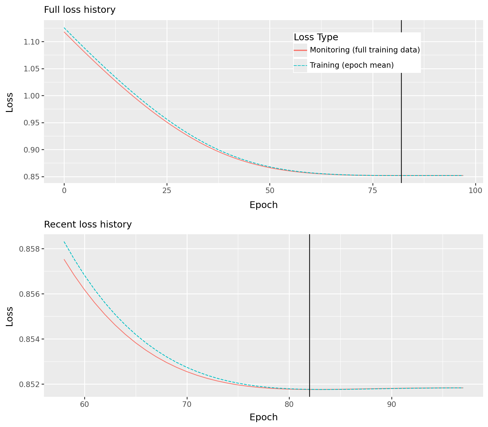
The overview shows the initial improvement and recent convergence. A flat curve does not by itself establish that the parameters are at an exact optimum.

Smooth noisy losses

Reuse the same model with minibatches and an EMA monitor:

result = opt.LieselOptim(
    model,
    optimizers=optax.adam(0.01),
    batch_size=32,
    loss_monitor=opt.EmaTrainLossMonitor(effective_window=2.0),
    stopper=stopper,
    show_progress=False,
    seed=42,
).fit()

result.plot_loss_overview()

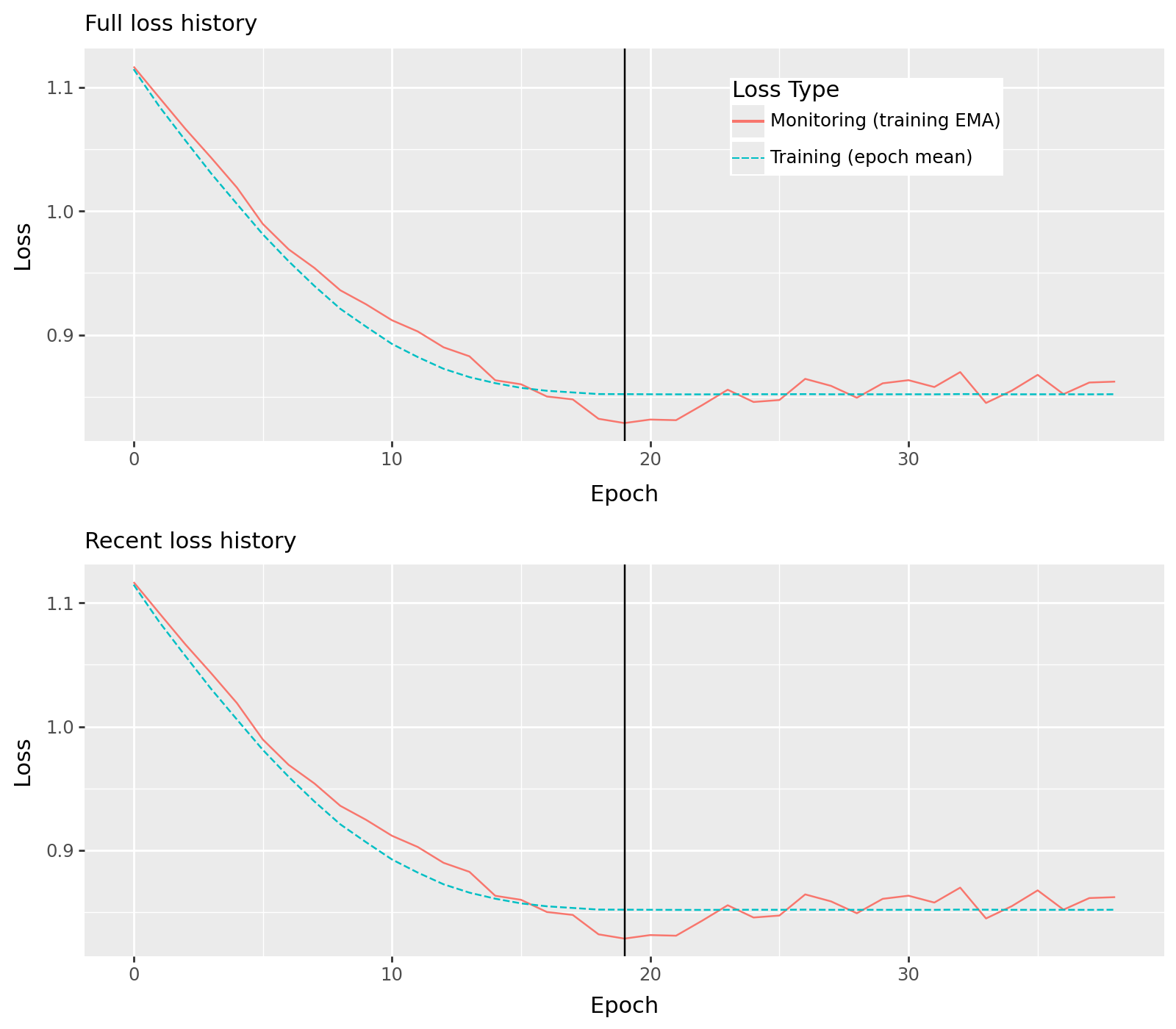
A larger effective_window smooths more and reacts more slowly. Its unit is an epoch’s worth of batches. Older losses fade gradually; they are not dropped at a fixed age. The average continues across epochs and reuses losses already computed for optimizer updates.

Because the average still includes older losses, it trails the current loss a little. The delay is about half the window: with effective_window=2.0, about one epoch. The default stopper of LieselOptim waits 10 epochs for an improvement, and the stopper above waits 20, so this delay makes little difference. Increase the window only if the monitored loss still jumps around near the end of the fit, and keep the delay well below how long the stopper waits.

An EMA combines losses from several parameter positions. Its best saved position is the snapshot at the end of that epoch; its exact loss need not equal the EMA monitor value. See EmaTrainLossMonitor for the formula and the alternative from_half_life() setting.

Investigate NaNs

For a configured LieselOptim builder, enable first-NaN reproduction capture on its engine before fitting:

engine = builder.build_engine()
engine.debug_nans = True
result = engine.fit()
debug_info = result.nan_debug

debug_info is None

True

If a NaN is detected, debug_info contains information for reproducing it; otherwise it is None. See OptimNaNDebugInfo for its contents. The captured information helps investigate the failure; it does not correct poor starting values.