PyMC and Liesel: Spike and Slab#
Liesel provides an interface for PyMC, a popular Python library for Bayesian Models. In this tutorial, we see how to specify a model in PyMC and then fit it using Liesel.
Be sure that you have pymc installed. If that’s not the case, you can
install Liesel with the optional dependency PyMC.
pip install liesel[pymc]
We will build a Spike and Slab model, a Bayesian approach that allows for variable selection by assuming a mixture of two distributions for the prior distribution of the regression coefficients: a point mass at zero (the “spike”) and a continuous distribution centered around zero (the “slab”). The model assumes that each coefficient \(\beta_j\) has a corresponding indicator variable \(\delta_j\) that takes a value of either 0 or 1, indicating whether the variable is included in the model or not. The prior distribution of the indicator variables is a Bernoulli distribution, with a parameter \(\theta\) that controls the sparsity of the model. When the parameter is close to 1, the model is more likely to include all variables, while when it is close to 0, the model is more likely to select only a few variables. In our case, we assign a Beta hyperprior to \(\theta\):
where \(\nu\) is a hyperparameter that we set to a fixed small value. That way, when \(\delta_j = 0\), the prior variance for \(\beta_j\) is extremely small, practically forcing it to be close to zero.
First, we generate the data. We use a model with four coefficients but assume that only two variables are relevant, namely the first and the third one.
RANDOM_SEED = 123
rng = np.random.RandomState(RANDOM_SEED)

n = 1000
p = 4

sigma_scalar = 1.0
beta_vec = np.array([3.0, 0.0, 4.0, 0.0])

X = rng.randn(n, p).astype(np.float32)

errors = rng.normal(size=n).astype(np.float32)

y = X @ beta_vec + sigma_scalar * errors
Then, we can specify the model using PyMC.
spike_and_slab_model = pm.Model()

mu = 0.0

alpha_tau = 1.0
beta_tau = 1.0

alpha_sigma = 1.0
beta_sigma = 1.0

alpha_theta = 8.0
beta_theta = 8.0

nu = 0.1

with spike_and_slab_model:
    # priors
    sigma2 = pm.InverseGamma("sigma2", alpha=alpha_sigma, beta=beta_sigma)

    theta = pm.Beta("theta", alpha=alpha_theta, beta=beta_theta)
    delta = pm.Bernoulli("delta", p=theta, size=p)
    tau = pm.InverseGamma("tau", alpha=alpha_tau, beta=beta_tau)

    beta = pm.Normal(
        "beta",
        mu=0.0,
        sigma=nu * (1 - delta) + delta * pm.math.sqrt(tau / sigma2),
        shape=p,
    )

    # make a data node
    Xx = pm.Data("X", X)

    # likelihood
    pm.Normal("y", mu=Xx @ beta, sigma=pm.math.sqrt(sigma2), observed=y)
Let’s take a look at our model:
spike_and_slab_model
The class PyMCInterface offers an interface between PyMC and
Goose. By default, the constructor of PyMCInterface keeps
track only of a representation of random variables that can be used in
sampling. For example, theta is transformed to the real-numbers space
with a log-odds transformation, and therefore the model only keeps track
of theta_log_odds__. However, we would like to access the
untransformed samples as well. We can do this by including them in the
additional_vars argument of the constructor of the interface.
The initial position can be extracted with get_initial_state().
The model state is represented as a Position.
interface = PyMCInterface(
    spike_and_slab_model, additional_vars=["sigma2", "tau", "theta"]
)
state = interface.get_initial_state()
Since \(\delta_j\) is a discrete variable, we need to use a Gibbs sampler to draw samples for it. Unfortunately, we cannot derive the posterior analytically, but what we can do is use a Metropolis-Hastings step as a transition function:
def delta_transition_fn(prng_key, model_state):
    draw_key, mh_key = jax.random.split(prng_key)
    theta_logodds = model_state["theta_logodds__"]
    p = jax.numpy.exp(theta_logodds) / (1 + jax.numpy.exp(theta_logodds))
    draw = jax.random.bernoulli(draw_key, p=p, shape=(4,))
    proposal = {"delta": jax.numpy.asarray(draw, dtype=np.int64)}
    _, state = gs.mh.mh_step(
        prng_key=mh_key, model=interface, proposal=proposal, model_state=model_state
    )
    return state
Finally, we can sample from the posterior as we do for any other Liesel
model. In this case, we use a GibbsKernel for
\(\boldsymbol{\delta}\) and a NUTSKernel both for the
remaining parameters.
builder = gs.EngineBuilder(seed=13, num_chains=4)
builder.set_model(interface)
builder.set_initial_values(state)
builder.set_duration(warmup_duration=1000, posterior_duration=2000)

builder.add_kernel(
    gs.NUTSKernel(
        position_keys=["beta", "sigma2_log__", "tau_log__", "theta_logodds__"]
    )
)
builder.add_kernel(gs.GibbsKernel(["delta"], transition_fn=delta_transition_fn))

builder.positions_included = ["sigma2", "tau"]

engine = builder.build()

engine.sample_all_epochs()
liesel.goose.builder - WARNING - No jitter functions provided. The initial values won't be jittered
liesel.goose.engine - INFO - Initializing kernels...
/Users/johannesbrachem/Documents/git/liesel/.venv/lib/python3.13/site-packages/jax/_src/numpy/array_methods.py:125: UserWarning: Explicitly requested dtype float64 requested in astype is not available, and will be truncated to dtype float32. To enable more dtypes, set the jax_enable_x64 configuration option or the JAX_ENABLE_X64 shell environment variable. See https://github.com/jax-ml/jax#current-gotchas for more.
  return lax_numpy.astype(self, dtype, copy=copy, device=device)
liesel.goose.engine - INFO - Done
liesel.goose.engine - INFO - Starting epoch: FAST_ADAPTATION, 75 transitions, 25 jitted together
  0%|                                                  | 0/3 [00:00<?, ?chunk/s]/var/folders/tn/j33340q16z763d6xp7mlcw4m0000gn/T/ipykernel_18448/3265445119.py:6: UserWarning: Explicitly requested dtype int64 requested in asarray is not available, and will be truncated to dtype int32. To enable more dtypes, set the jax_enable_x64 configuration option or the JAX_ENABLE_X64 shell environment variable. See https://github.com/jax-ml/jax#current-gotchas for more.
  proposal = {"delta": jax.numpy.asarray(draw, dtype=np.int64)}
 33%|██████████████                            | 1/3 [00:02<00:04,  2.24s/chunk]100%|██████████████████████████████████████████| 3/3 [00:02<00:00,  1.34chunk/s]
liesel.goose.engine - WARNING - Errors per chain for kernel_00: 3, 2, 3, 4 / 75 transitions
liesel.goose.engine - INFO - Finished epoch
liesel.goose.engine - INFO - Starting epoch: SLOW_ADAPTATION, 25 transitions, 25 jitted together
  0%|                                                  | 0/1 [00:00<?, ?chunk/s]100%|████████████████████████████████████████| 1/1 [00:00<00:00, 1475.31chunk/s]
liesel.goose.engine - WARNING - Errors per chain for kernel_00: 1, 1, 1, 1 / 25 transitions
liesel.goose.engine - INFO - Finished epoch
liesel.goose.engine - INFO - Starting epoch: SLOW_ADAPTATION, 50 transitions, 25 jitted together
  0%|                                                  | 0/2 [00:00<?, ?chunk/s]100%|████████████████████████████████████████| 2/2 [00:00<00:00, 2554.39chunk/s]
liesel.goose.engine - INFO - Finished epoch
liesel.goose.engine - INFO - Starting epoch: SLOW_ADAPTATION, 100 transitions, 25 jitted together
  0%|                                                  | 0/4 [00:00<?, ?chunk/s]100%|████████████████████████████████████████| 4/4 [00:00<00:00, 3023.47chunk/s]
liesel.goose.engine - WARNING - Errors per chain for kernel_00: 1, 2, 1, 1 / 100 transitions
liesel.goose.engine - INFO - Finished epoch
liesel.goose.engine - INFO - Starting epoch: SLOW_ADAPTATION, 200 transitions, 25 jitted together
  0%|                                                  | 0/8 [00:00<?, ?chunk/s]100%|█████████████████████████████████████████| 8/8 [00:00<00:00, 978.61chunk/s]
liesel.goose.engine - WARNING - Errors per chain for kernel_00: 1, 1, 1, 1 / 200 transitions
liesel.goose.engine - INFO - Finished epoch
liesel.goose.engine - INFO - Starting epoch: SLOW_ADAPTATION, 500 transitions, 25 jitted together
  0%|                                                 | 0/20 [00:00<?, ?chunk/s]100%|███████████████████████████████████████| 20/20 [00:00<00:00, 348.66chunk/s]
liesel.goose.engine - WARNING - Errors per chain for kernel_00: 1, 1, 1, 3 / 500 transitions
liesel.goose.engine - INFO - Finished epoch
liesel.goose.engine - INFO - Starting epoch: FAST_ADAPTATION, 50 transitions, 25 jitted together
  0%|                                                  | 0/2 [00:00<?, ?chunk/s]100%|████████████████████████████████████████| 2/2 [00:00<00:00, 2427.26chunk/s]
liesel.goose.engine - WARNING - Errors per chain for kernel_00: 1, 1, 1, 1 / 50 transitions
liesel.goose.engine - INFO - Finished epoch
liesel.goose.engine - INFO - Finished warmup
liesel.goose.engine - INFO - Starting epoch: POSTERIOR, 2000 transitions, 25 jitted together
  0%|                                                 | 0/80 [00:00<?, ?chunk/s] 41%|████████████████                       | 33/80 [00:00<00:00, 329.42chunk/s] 82%|████████████████████████████████▏      | 66/80 [00:00<00:00, 289.79chunk/s]100%|███████████████████████████████████████| 80/80 [00:00<00:00, 290.03chunk/s]
liesel.goose.engine - INFO - Finished epoch
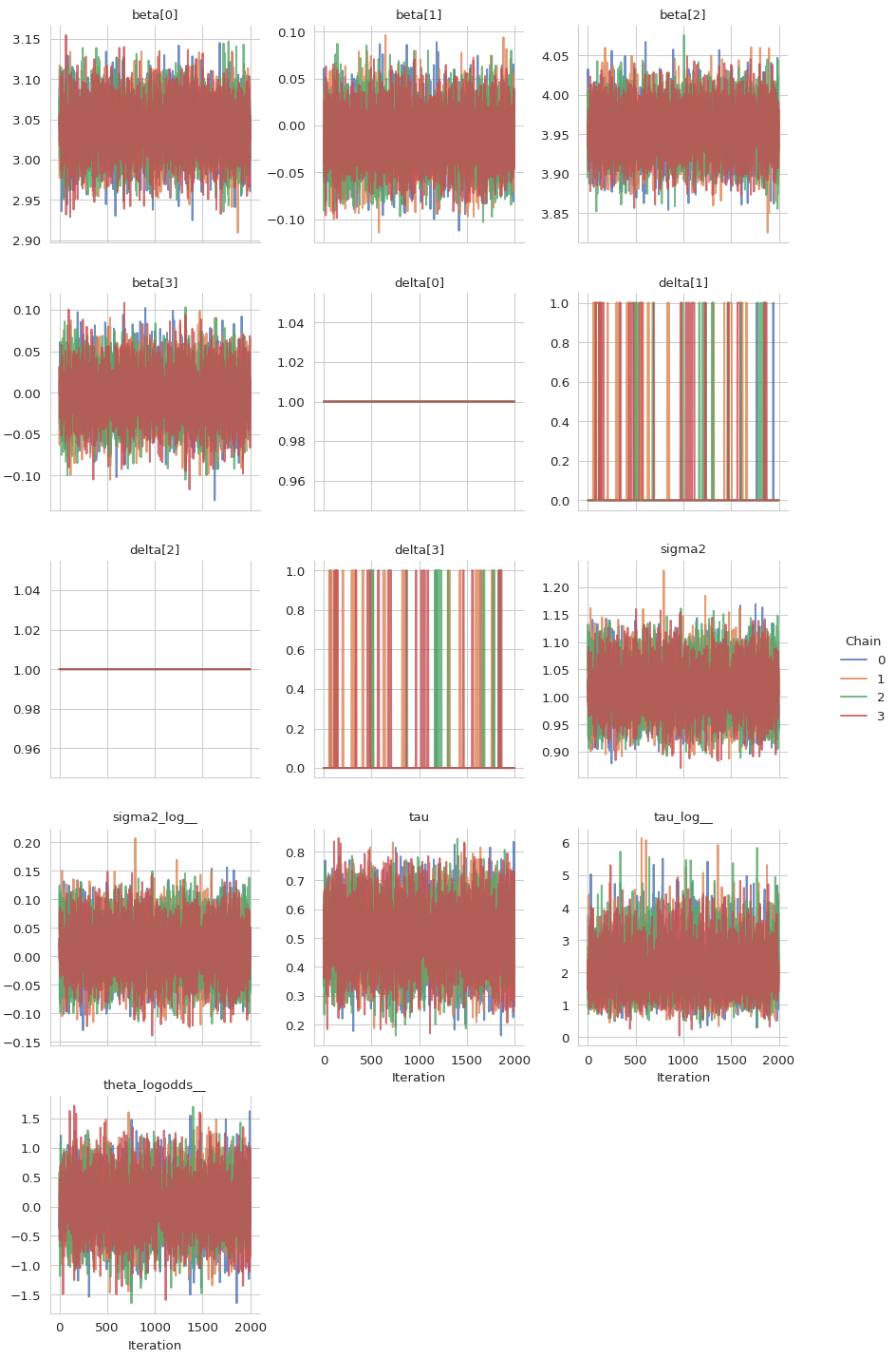
Now, we can take a look at the summary of the results and at the trace plots.
results = engine.get_results()
print(gs.Summary(results))
/Users/johannesbrachem/Documents/git/liesel/.venv/lib/python3.13/site-packages/arviz/stats/diagnostics.py:845: RuntimeWarning: invalid value encountered in scalar divide
  varsd = varvar / evar / 4
/Users/johannesbrachem/Documents/git/liesel/.venv/lib/python3.13/site-packages/arviz/stats/diagnostics.py:845: RuntimeWarning: invalid value encountered in scalar divide
  varsd = varvar / evar / 4
/Users/johannesbrachem/Documents/git/liesel/.venv/lib/python3.13/site-packages/arviz/stats/diagnostics.py:596: RuntimeWarning: invalid value encountered in scalar divide
  (between_chain_variance / within_chain_variance + num_samples - 1) / (num_samples)

                         var_fqn     kernel var_index  sample_size      mean  \
variable
beta                     beta[0]  kernel_00      (0,)         8000  3.037814
beta                     beta[1]  kernel_00      (1,)         8000 -0.010874
beta                     beta[2]  kernel_00      (2,)         8000  3.955981
beta                     beta[3]  kernel_00      (3,)         8000 -0.001599
delta                   delta[0]  kernel_01      (0,)         8000  1.000000
delta                   delta[1]  kernel_01      (1,)         8000  0.076625
delta                   delta[2]  kernel_01      (2,)         8000  1.000000
delta                   delta[3]  kernel_01      (3,)         8000  0.052375
sigma2                    sigma2          -        ()         8000  1.014596
sigma2_log__        sigma2_log__  kernel_00        ()         8000  0.013453
tau                          tau          -        ()         8000  0.506953
tau_log__              tau_log__  kernel_00        ()         8000  2.154096
theta_logodds__  theta_logodds__  kernel_00        ()         8000  0.029387

                      var        sd      ess_bulk     ess_tail  mcse_mean  \
variable
beta             0.001058  0.032525  12613.238337  6099.070961   0.000289
beta             0.000886  0.029769  12218.425015  6130.544738   0.000269
beta             0.000985  0.031387  13606.196293  6070.164816   0.000269
beta             0.000955  0.030897  13043.404768  6038.970396   0.000271
delta            0.000000  0.000000   8000.000000  8000.000000   0.000000
delta            0.070754  0.265996    319.840916   319.840916   0.014874
delta            0.000000  0.000000   8000.000000  8000.000000   0.000000
delta            0.049632  0.222782    562.970934   562.970934   0.009390
sigma2           0.002140  0.046265  11878.389693  5810.568129   0.000427
sigma2_log__     0.002073  0.045534  11878.392996  5810.568129   0.000418
tau              0.012417  0.111432   7248.664938  5306.853795   0.001313
tau_log__        0.623456  0.789592   7909.243715  4692.050581   0.009597
theta_logodds__  0.220301  0.469362   7248.663353  5306.853795   0.005503

                  mcse_sd      rhat    q_0.05     q_0.5    q_0.95   hdi_low  \
variable
beta             0.000386  1.000295  2.985235  3.037885  3.091991  2.984958
beta             0.000340  1.000364 -0.060268 -0.010704  0.037495 -0.062392
beta             0.000354  1.000310  3.904037  3.956081  4.007212  3.904486
beta             0.000362  1.000296 -0.052088 -0.001520  0.049825 -0.051128
delta                 NaN       NaN  1.000000  1.000000  1.000000  1.000000
delta            0.023673  1.023458  0.000000  0.000000  1.000000  0.000000
delta                 NaN       NaN  1.000000  1.000000  1.000000  1.000000
delta            0.018866  1.010037  0.000000  0.000000  1.000000  0.000000
sigma2           0.000567  1.001344  0.940747  1.012874  1.094405  0.938549
sigma2_log__     0.000552  1.001313 -0.061081  0.012792  0.090210 -0.058979
tau              0.001279  1.001675  0.322230  0.506900  0.688730  0.323917
tau_log__        0.010454  1.001987  1.026337  2.054462  3.591636  0.875061
theta_logodds__  0.005829  1.001682 -0.743543  0.027600  0.794188 -0.735829

                 hdi_high
variable
beta             3.091510
beta             0.035103
beta             4.007542
beta             0.050621
delta            1.000000
delta            0.000000
delta            1.000000
delta            0.000000
sigma2           1.092050
sigma2_log__     0.092068
tau              0.689343
tau_log__        3.353702
theta_logodds__  0.797049
As we can see from the posterior means of the \(\boldsymbol{\delta}\) parameters, the model was able to recognize those variable with no influence on the respose \(\mathbf{y}\):
\(\delta_1\) and \(\delta_3\) (
delta[0]anddelta[2]in the table) have a posterior mean of \(1\), indicating inclusion.\(\delta_2\) and \(\delta_4\) (
delta[1]anddelta[3]in the table) have a posterior mean of \(0.06\), indicating exclusion.
gs.plot_trace(results)