GEV responses#

In this tutorial, we illustrate how to set up a distributional regression model with the generalized extreme value distribution as a response distribution. We configure the model in Python with Liesel-GAM, using liesel_gam.TermBuilder for linear terms and P-splines. See the Liesel-GAM documentation and examples for a broader overview of the available term types.

We simulate data from a GEV model with three distributional parameters:

The location parameter ($\mu$) is a function of an intercept and a non-linear covariate effect.
The scale parameter ($\sigma$) is a function of an intercept and a linear effect and uses a log-link.
The shape or concentration parameter ($\xi$) is a function of an intercept and a linear effect.

import jax
import jax.numpy as jnp
import matplotlib.pyplot as plt
import numpy as np
import seaborn as sns
import tensorflow_probability.substrates.jax.distributions as tfd

import liesel.goose as gs
import liesel.model as lsl
import liesel_gam as gam

sns.set_theme(style="whitegrid")

Warning message:
package ‘arrow’ was built under R version 4.5.2

key = jax.random.PRNGKey(13)
n = 500

key, key_x0, key_x1, key_x2, key_y = jax.random.split(key, 5)

x0 = jax.random.uniform(key_x0, (n,))
x1 = jax.random.uniform(key_x1, (n,))
x2 = jax.random.uniform(key_x2, (n,))

true_loc = jnp.sin(2 * jnp.pi * x0)
true_scale = jnp.exp(-1.0 + x1)
true_concentration = 0.1 + x2

y = tfd.GeneralizedExtremeValue(
    loc=true_loc,
    scale=true_scale,
    concentration=true_concentration,
).sample(seed=key_y)

data = pd.DataFrame({
    "y": np.asarray(y),
    "intercept": np.ones_like(y),
    "x0": np.asarray(x0),
    "x1": np.asarray(x1),
    "x2": np.asarray(x2),
    "true_loc": np.asarray(true_loc),
    "true_scale": np.asarray(true_scale),
    "true_concentration": np.asarray(true_concentration),
})

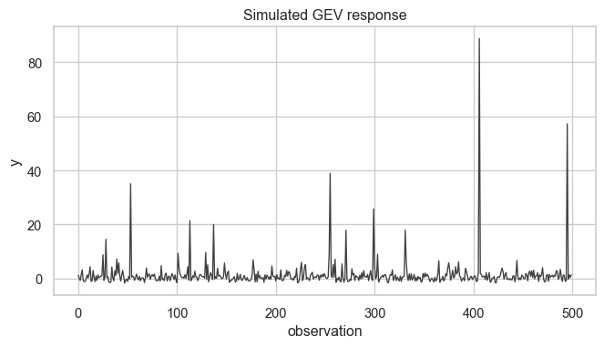
Here is the simulated response:

fig, ax = plt.subplots(figsize=(8, 4))
sns.lineplot(x=data.index, y=data["y"], ax=ax, color="0.25", linewidth=1)
ax.set(xlabel="observation", ylabel="y", title="Simulated GEV response")
plt.show()

../../_images/plot-data-output-11.png

We now construct the distributional regression model. The TermBuilder reads the covariates from a pandas data frame and creates Liesel variables for the corresponding model terms. The additive predictors are passed directly to tfd.GeneralizedExtremeValue.

tb = gam.TermBuilder.from_df(data, default_inference=gs.MCMCSpec(gs.IWLSKernel))

loc = gam.AdditivePredictor("loc", intercept=True)
scale = gam.AdditivePredictor("scale", inv_link=jnp.exp, intercept=False)
concentration = gam.AdditivePredictor("concentration", intercept=False)

loc_smooth = tb.ps("x0", k=10)
scale_x1 = tb.lin("intercept + x1")
concentration_x2 = tb.lin("intercept + x2")

loc += loc_smooth
scale += scale_x1
concentration += concentration_x2

# The GEV distribution is numerically delicate around xi = 0, so we start away
# from the Gumbel case while keeping the linear effect initialized at zero.
concentration_x2.coef.value = jnp.array([0.1, 0.0])
concentration.update()

response_dist = lsl.Dist(
    tfd.GeneralizedExtremeValue,
    loc=loc,
    scale=scale,
    concentration=concentration,
)
y_var = lsl.Var.new_obs(data["y"].to_numpy(), response_dist, name="y")

model = lsl.Model([y_var])

# ScaleIG represents tau = sqrt(tau2). The Gibbs kernel samples tau2.
loc_smooth_tau2_name = loc_smooth.scale.value_node[0].name

We use Liesel’s MCMCSpec objects, which are added automatically by Liesel-GAM, to set up the sampler. The default Liesel-GAM setup uses IWLS kernels for regression coefficients and a Gibbs kernel for the smoothing variance of the P-spline.

The support of the GEV distribution changes with the parameter values (compare Wikipedia).

results = gs.LieselMCMC(model).run_for_epochs(
    seed=1, num_chains=4, adaptation=1000, posterior=2500
)
gs.Summary(results)

liesel.goose.builder - WARNING - No jitter functions provided for position keys '$\\beta_{ps(x0)}$', '$\\tau_{ps(x0)}^2$', '$\\beta_{0,loc}$', '$\\beta_{lin(X)}$', '$\\beta_{lin(X1)}$'. The initial values for these keys won't be jittered
liesel.goose.engine - INFO - Initializing kernels...
liesel.goose.engine - INFO - Done
liesel.goose.engine - INFO - Starting epoch: FAST_ADAPTATION, 100 transitions, 25 jitted together
  0%|                                                  | 0/4 [00:00<?, ?chunk/s] 25%|██████████▌                               | 1/4 [00:03<00:10,  3.62s/chunk]100%|██████████████████████████████████████████| 4/4 [00:03<00:00,  1.10chunk/s]
liesel.goose.engine - WARNING - Errors per chain for kernel_00: 1, 1, 1, 1 / 100 transitions
liesel.goose.engine - WARNING - Errors per chain for kernel_03: 2, 0, 0, 2 / 100 transitions
liesel.goose.engine - WARNING - Errors per chain for kernel_04: 3, 4, 2, 2 / 100 transitions
liesel.goose.engine - INFO - Finished epoch
liesel.goose.engine - INFO - Starting epoch: SLOW_ADAPTATION, 25 transitions, 25 jitted together
  0%|                                                  | 0/1 [00:00<?, ?chunk/s]100%|████████████████████████████████████████| 1/1 [00:00<00:00, 1217.86chunk/s]
liesel.goose.engine - WARNING - Errors per chain for kernel_00: 1, 2, 1, 1 / 25 transitions
liesel.goose.engine - WARNING - Errors per chain for kernel_03: 1, 1, 0, 1 / 25 transitions
liesel.goose.engine - WARNING - Errors per chain for kernel_04: 1, 1, 1, 1 / 25 transitions
liesel.goose.engine - INFO - Finished epoch
liesel.goose.engine - INFO - Starting epoch: SLOW_ADAPTATION, 50 transitions, 25 jitted together
  0%|                                                  | 0/2 [00:00<?, ?chunk/s]100%|████████████████████████████████████████| 2/2 [00:00<00:00, 1455.85chunk/s]
liesel.goose.engine - WARNING - Errors per chain for kernel_00: 1, 1, 1, 0 / 50 transitions
liesel.goose.engine - WARNING - Errors per chain for kernel_03: 2, 0, 0, 3 / 50 transitions
liesel.goose.engine - WARNING - Errors per chain for kernel_04: 1, 1, 1, 2 / 50 transitions
liesel.goose.engine - INFO - Finished epoch
liesel.goose.engine - INFO - Starting epoch: SLOW_ADAPTATION, 100 transitions, 25 jitted together
  0%|                                                  | 0/4 [00:00<?, ?chunk/s]100%|████████████████████████████████████████| 4/4 [00:00<00:00, 1801.87chunk/s]
liesel.goose.engine - WARNING - Errors per chain for kernel_00: 1, 1, 2, 0 / 100 transitions
liesel.goose.engine - WARNING - Errors per chain for kernel_03: 2, 1, 0, 1 / 100 transitions
liesel.goose.engine - WARNING - Errors per chain for kernel_04: 3, 1, 2, 1 / 100 transitions
liesel.goose.engine - INFO - Finished epoch
liesel.goose.engine - INFO - Starting epoch: SLOW_ADAPTATION, 525 transitions, 25 jitted together
  0%|                                                 | 0/21 [00:00<?, ?chunk/s] 76%|█████████████████████████████▋         | 16/21 [00:00<00:00, 157.53chunk/s]100%|███████████████████████████████████████| 21/21 [00:00<00:00, 131.69chunk/s]
liesel.goose.engine - WARNING - Errors per chain for kernel_00: 1, 2, 1, 1 / 525 transitions
liesel.goose.engine - WARNING - Errors per chain for kernel_03: 4, 1, 2, 1 / 525 transitions
liesel.goose.engine - WARNING - Errors per chain for kernel_04: 7, 6, 8, 4 / 525 transitions
liesel.goose.engine - INFO - Finished epoch
liesel.goose.engine - INFO - Starting epoch: FAST_ADAPTATION, 200 transitions, 25 jitted together
  0%|                                                  | 0/8 [00:00<?, ?chunk/s]100%|█████████████████████████████████████████| 8/8 [00:00<00:00, 623.89chunk/s]
liesel.goose.engine - WARNING - Errors per chain for kernel_00: 2, 1, 1, 3 / 200 transitions
liesel.goose.engine - WARNING - Errors per chain for kernel_03: 1, 3, 3, 2 / 200 transitions
liesel.goose.engine - WARNING - Errors per chain for kernel_04: 2, 4, 84, 2 / 200 transitions
liesel.goose.engine - INFO - Finished epoch
liesel.goose.engine - INFO - Finished warmup
liesel.goose.engine - INFO - Starting epoch: POSTERIOR, 2500 transitions, 25 jitted together
  0%|                                                | 0/100 [00:00<?, ?chunk/s] 17%|██████▍                               | 17/100 [00:00<00:00, 156.17chunk/s] 33%|████████████▌                         | 33/100 [00:00<00:00, 103.29chunk/s] 45%|█████████████████▌                     | 45/100 [00:00<00:00, 95.92chunk/s] 56%|█████████████████████▊                 | 56/100 [00:00<00:00, 70.69chunk/s] 66%|█████████████████████████▋             | 66/100 [00:00<00:00, 75.90chunk/s] 76%|█████████████████████████████▋         | 76/100 [00:00<00:00, 81.03chunk/s] 85%|█████████████████████████████████▏     | 85/100 [00:00<00:00, 82.51chunk/s] 94%|████████████████████████████████████▋  | 94/100 [00:01<00:00, 83.47chunk/s]100%|██████████████████████████████████████| 100/100 [00:01<00:00, 85.17chunk/s]
liesel.goose.engine - WARNING - Errors per chain for kernel_04: 8, 4, 872, 2 / 2500 transitions
liesel.goose.engine - INFO - Finished epoch

Parameter summary:

		kernel	mean	sd	q_0.05	q_0.5	q_0.95	sample_size	ess_bulk	ess_tail	rhat
parameter	index
$\beta_{0,loc}$	()	kernel_02	0.003	0.026	-0.037	0.002	0.047	10000	177.883	457.979	1.021
$\beta_{lin(X)}$	(0,)	kernel_03	-1.218	0.099	-1.378	-1.219	-1.054	10000	202.379	508.367	1.018
$\beta_{lin(X)}$	(1,)	kernel_03	1.400	0.137	1.172	1.399	1.623	10000	307.969	865.843	1.006
$\beta_{lin(X1)}$	(0,)	kernel_04	0.071	0.110	-0.061	0.074	0.255	10000	8.659	50.997	1.406
$\beta_{lin(X1)}$	(1,)	kernel_04	1.070	0.201	0.724	1.075	1.296	10000	10.591	678.843	1.320
$\beta_{ps(x0)}$	(0,)	kernel_00	0.081	0.117	-0.112	0.082	0.271	10000	256.969	495.439	1.029
	(1,)	kernel_00	0.002	0.119	-0.194	0.006	0.187	10000	373.587	726.253	1.009
	(2,)	kernel_00	0.048	0.125	-0.161	0.047	0.256	10000	309.323	560.738	1.005
	(3,)	kernel_00	-0.008	0.110	-0.185	-0.005	0.163	10000	328.177	556.151	1.008
	(4,)	kernel_00	-0.149	0.102	-0.314	-0.149	0.021	10000	300.963	548.966	1.019
	(5,)	kernel_00	0.042	0.072	-0.076	0.041	0.157	10000	296.677	530.711	1.021
	(6,)	kernel_00	-0.357	0.048	-0.437	-0.356	-0.281	10000	303.546	527.516	1.019
	(7,)	kernel_00	-0.000	0.020	-0.034	0.000	0.032	10000	312.715	543.417	1.006
	(8,)	kernel_00	-0.050	0.060	-0.145	-0.050	0.050	10000	296.621	421.972	1.025
$\tau_{ps(x0)}^2$	()	kernel_01	0.031	0.022	0.012	0.025	0.068	10000	1540.702	2724.639	1.003

Acceptance probabilities:

			acceptance_probability	position_moved
kernel	positions	phase
kernel_00	$\beta_{ps(x0)}$	posterior	0.828	0.823
kernel_00	$\beta_{ps(x0)}$	warmup	0.793	0.792
kernel_01	$\tau_{ps(x0)}^2$	posterior	1.000	1.000
kernel_01	$\tau_{ps(x0)}^2$	warmup	1.000	1.000
kernel_02	$\beta_{0,loc}$	posterior	0.882	0.882
kernel_02	$\beta_{0,loc}$	warmup	0.888	0.886
kernel_03	$\beta_{lin(X)}$	posterior	0.867	0.866
kernel_03	$\beta_{lin(X)}$	warmup	0.793	0.790
kernel_04	$\beta_{lin(X1)}$	posterior	0.848	0.848
kernel_04	$\beta_{lin(X1)}$	warmup	0.791	0.793

Error summary:

					count	sample_size	sample_size_total	relative
kernel	positions	error_code	error_msg	phase
kernel_00	$\beta_{ps(x0)}$	90	nan acceptance prob	warmup	28	4000	4000	0.007
kernel_00	$\beta_{ps(x0)}$	90	nan acceptance prob	posterior	0	10000	10000	0.000
kernel_03	$\beta_{lin(X)}$	90	nan acceptance prob	warmup	33	4000	4000	0.008
kernel_03	$\beta_{lin(X)}$	90	nan acceptance prob	posterior	0	10000	10000	0.000
kernel_04	$\beta_{lin(X1)}$	2	indefinite information matrix (fallback to identity)	warmup	84	4000	4000	0.021
		2	indefinite information matrix (fallback to identity)	posterior	872	10000	10000	0.087
		90	nan acceptance prob	warmup	58	4000	4000	0.014
		90	nan acceptance prob	posterior	0	10000	10000	0.000
		92	indefinite information matrix (fallback to identity) + nan acceptance prob	warmup	2	4000	4000	0.001
		92		posterior	14	10000	10000	0.001

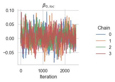
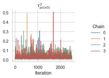
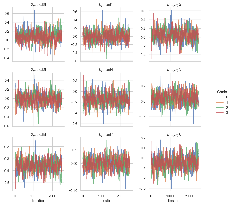
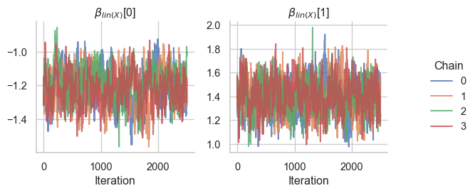
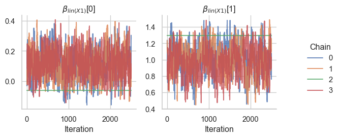
The corresponding trace plots:

gs.plot_trace(results, loc.intercept.name)
gs.plot_trace(results, loc_smooth_tau2_name)
gs.plot_trace(results, loc_smooth.coef.name)
gs.plot_trace(results, scale_x1.coef.name)
gs.plot_trace(results, concentration_x2.coef.name)

../../_images/traces-output-1.png

../../_images/traces-output-2.png

../../_images/traces-output-3.png

../../_images/traces-output-4.png

../../_images/traces-output-5.png

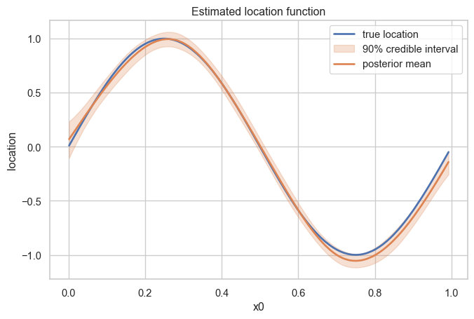
Finally, we can evaluate the posterior samples of the location predictor and compare the posterior mean with the true function used in the simulation.

samples = results.get_posterior_samples()
loc_samples = model.vars["loc"].predict(samples)
loc_summary = gs.SamplesSummary.from_array(
    loc_samples,
    name="loc",
    which=["mean", "quantiles"],
)
loc_summary_df = loc_summary.to_dataframe().reset_index()

loc_summary_df["x0"] = data["x0"].to_numpy()
loc_summary_df["true_loc"] = data["true_loc"].to_numpy()
loc_summary_df = loc_summary_df.sort_values("x0")

fig, ax = plt.subplots(figsize=(8, 5))
sns.lineplot(
    data=loc_summary_df,
    x="x0",
    y="true_loc",
    color=sns.color_palette()[0],
    linewidth=2,
    label="true location",
    ax=ax,
)
ax.fill_between(
    loc_summary_df["x0"],
    loc_summary_df["q_0.05"],
    loc_summary_df["q_0.95"],
    color=sns.color_palette()[1],
    alpha=0.25,
    label="90% credible interval",
)
sns.lineplot(
    data=loc_summary_df,
    x="x0",
    y="mean",
    color=sns.color_palette()[1],
    linewidth=2,
    label="posterior mean",
    ax=ax,
)

ax.set(xlabel="x0", ylabel="location", title="Estimated location function")
plt.show()

../../_images/spline-output-1.png