Parameter transformations

This tutorial builds on the linear regression tutorial. Here, we demonstrate how to transform a positive-valued parameter so that it can be sampled with a NUTS kernel on an unconstrained scale.

First, let’s set up the linear regression model again. The data-generating process and the model structure are the same as in the linear regression tutorial, but this time we prepare the model for joint NUTS sampling of the regression coefficients and the error variance.

import jax
import jax.numpy as jnp
import numpy as np
import matplotlib.pyplot as plt

# We use distributions and bijectors from tensorflow probability
import tensorflow_probability.substrates.jax.distributions as tfd
import tensorflow_probability.substrates.jax.bijectors as tfb

import liesel.goose as gs
import liesel.model as lsl

rng = np.random.default_rng(42)

# data-generating process
n = 500
true_beta = np.array([1.0, 2.0])
true_sigma = 1.0
x0 = rng.uniform(size=n)
X_mat = np.c_[np.ones(n), x0]
y_vec = X_mat @ true_beta + rng.normal(scale=true_sigma, size=n)

# Model
# Part 1: Model for the mean
beta_prior = lsl.Dist(tfd.Normal, loc=0.0, scale=100.0)
beta = lsl.Var.new_param(
    value=np.array([0.0, 0.0]),
    dist=beta_prior,
    name="beta",
    inference=gs.MCMCSpec(gs.NUTSKernel, kernel_group="1"),
)

X = lsl.Var.new_obs(X_mat, name="X")
mu = lsl.Var(lsl.Calc(jnp.dot, X, beta), name="mu")

# Part 2: Model for the standard deviation
a = lsl.Var(0.01, name="a")
b = lsl.Var(0.01, name="b")
sigma_sq_prior = lsl.Dist(tfd.InverseGamma, concentration=a, scale=b)
sigma_sq = lsl.Var.new_param(value=10.0, dist=sigma_sq_prior, name="sigma_sq")

sigma = lsl.Var(lsl.Calc(jnp.sqrt, sigma_sq), name="sigma")

# Observation model
y_dist = lsl.Dist(tfd.Normal, loc=mu, scale=sigma)
y = lsl.Var(y_vec, dist=y_dist, name="y")

Now let’s try to sample the regression coefficients \(\boldsymbol{\beta}\) and the variance \(\sigma^2\) with a single NUTS kernel. NUTS operates on unconstrained real-valued parameters, whereas \(\sigma^2\) must remain positive. We therefore biject sigma_sq with an exponential bijector. This creates an unconstrained latent variable representing \(\log(\sigma^2)\) and keeps sigma_sq as the positive back-transformed value. Both beta and the transformed variance receive NUTS inference specifications with the same kernel_group, so Goose samples them jointly in one NUTS block.

sigma_sq.biject(tfb.Exp(), inference=gs.MCMCSpec(gs.NUTSKernel, kernel_group="1"))

model = lsl.Model(y)
model.plot()

liesel.model.model - WARNING - Inconsistent log prob decomposition: Model.log_prob=-1177.35 ≠ (Model.log_lik=0.00 + Model.log_prior=-15.72).
liesel.model.model - WARNING - Var(name="y") has a distribution but Var.parameter=False and Var.observed=False.

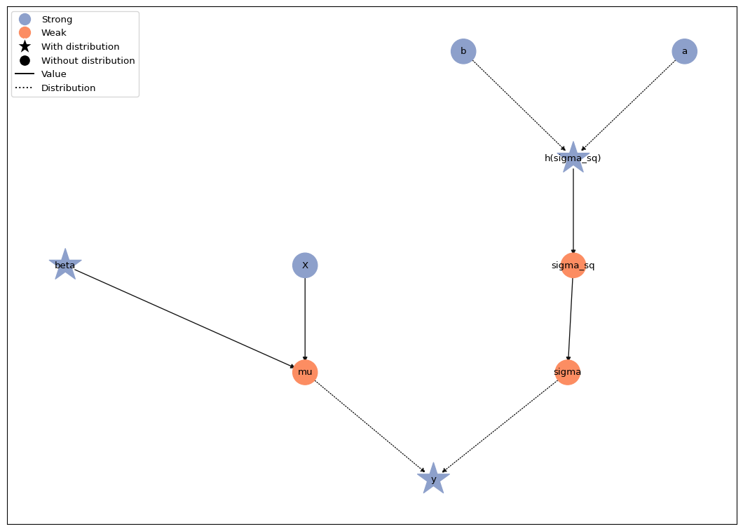
The response distribution still requires the standard deviation on the original scale. The model graph shows that sigma_sq is now a deterministic, positive-valued transformation of its unconstrained latent variable. The standard deviation sigma is then computed as sqrt(sigma_sq), so the likelihood continues to receive a valid scale parameter.

Now we can set up and run the MCMC algorithm directly from the MCMCSpec objects stored in the model. We also include sigma_sq in the stored positions, because the NUTS kernel itself samples the transformed variable, while sigma_sq is the easier quantity to interpret.

results = gs.LieselMCMC(model).run_for_epochs(
    seed=1,
    num_chains=4,
    adaptation=1000,
    posterior=1000,
    positions_included=["sigma_sq"],
)

liesel.goose.builder - WARNING - No jitter functions provided for position keys 'h(sigma_sq)', 'beta'. The initial values for these keys won't be jittered
liesel.goose.engine - INFO - Initializing kernels...
liesel.goose.engine - INFO - Done
liesel.goose.engine - INFO - Starting epoch: FAST_ADAPTATION, 100 transitions, 25 jitted together
  0%|                                                  | 0/4 [00:00<?, ?chunk/s] 25%|██████████▌                               | 1/4 [00:01<00:04,  1.38s/chunk]100%|██████████████████████████████████████████| 4/4 [00:01<00:00,  2.89chunk/s]
liesel.goose.engine - WARNING - Errors per chain for kernel_00: 1, 1, 2, 4 / 100 transitions
liesel.goose.engine - INFO - Finished epoch
liesel.goose.engine - INFO - Starting epoch: SLOW_ADAPTATION, 25 transitions, 25 jitted together
  0%|                                                  | 0/1 [00:00<?, ?chunk/s]100%|████████████████████████████████████████| 1/1 [00:00<00:00, 1240.55chunk/s]
liesel.goose.engine - WARNING - Errors per chain for kernel_00: 2, 1, 2, 1 / 25 transitions
liesel.goose.engine - INFO - Finished epoch
liesel.goose.engine - INFO - Starting epoch: SLOW_ADAPTATION, 50 transitions, 25 jitted together
  0%|                                                  | 0/2 [00:00<?, ?chunk/s]100%|████████████████████████████████████████| 2/2 [00:00<00:00, 1683.78chunk/s]
liesel.goose.engine - WARNING - Errors per chain for kernel_00: 2, 3, 1, 2 / 50 transitions
liesel.goose.engine - INFO - Finished epoch
liesel.goose.engine - INFO - Starting epoch: SLOW_ADAPTATION, 100 transitions, 25 jitted together
  0%|                                                  | 0/4 [00:00<?, ?chunk/s]100%|████████████████████████████████████████| 4/4 [00:00<00:00, 2899.12chunk/s]
liesel.goose.engine - WARNING - Errors per chain for kernel_00: 2, 2, 2, 2 / 100 transitions
liesel.goose.engine - INFO - Finished epoch
liesel.goose.engine - INFO - Starting epoch: SLOW_ADAPTATION, 525 transitions, 25 jitted together
  0%|                                                 | 0/21 [00:00<?, ?chunk/s]100%|███████████████████████████████████████| 21/21 [00:00<00:00, 303.84chunk/s]
liesel.goose.engine - WARNING - Errors per chain for kernel_00: 1, 3, 3, 3 / 525 transitions
liesel.goose.engine - INFO - Finished epoch
liesel.goose.engine - INFO - Starting epoch: FAST_ADAPTATION, 200 transitions, 25 jitted together
  0%|                                                  | 0/8 [00:00<?, ?chunk/s]100%|█████████████████████████████████████████| 8/8 [00:00<00:00, 895.45chunk/s]
liesel.goose.engine - WARNING - Errors per chain for kernel_00: 2, 4, 3, 1 / 200 transitions
liesel.goose.engine - INFO - Finished epoch
liesel.goose.engine - INFO - Finished warmup
liesel.goose.engine - INFO - Starting epoch: POSTERIOR, 1000 transitions, 25 jitted together
  0%|                                                 | 0/40 [00:00<?, ?chunk/s] 80%|███████████████████████████████▏       | 32/40 [00:00<00:00, 307.02chunk/s]100%|███████████████████████████████████████| 40/40 [00:00<00:00, 291.56chunk/s]
liesel.goose.engine - INFO - Finished epoch

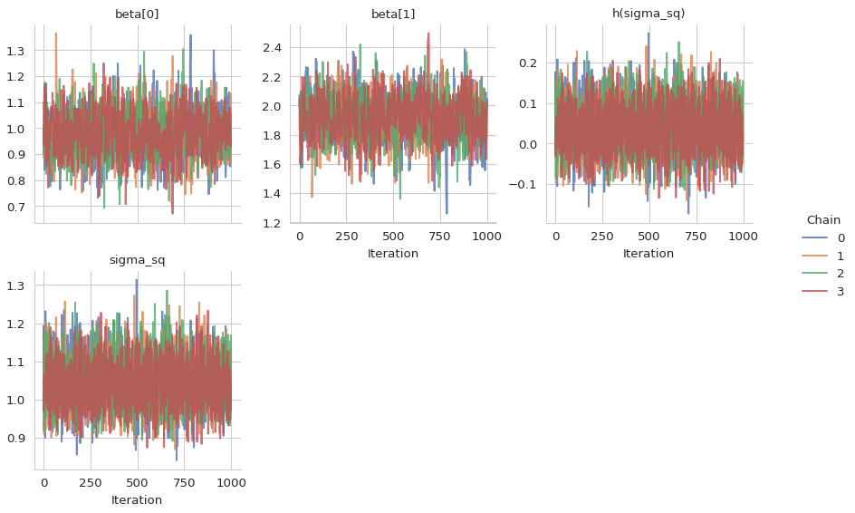
Judging from the trace plots, it seems that all chains have converged.

gs.plot_trace(results)

We can also take a look at the summary table, which includes both the original \(\sigma^2\) and the transformed \(\log(\sigma^2)\).

gs.Summary(results)

Parameter summary:

		kernel	mean	sd	q_0.05	q_0.5	q_0.95	sample_size	ess_bulk	ess_tail	rhat
parameter	index
beta	(0,)	kernel_00	0.981	0.091	0.833	0.980	1.130	4000	816.958	1116.378	1.002
	(1,)	kernel_00	1.914	0.159	1.656	1.916	2.173	4000	772.001	917.470	1.001
h(sigma_sq)	()	kernel_00	0.042	0.062	-0.058	0.040	0.145	4000	5406.551	3299.936	1.001
sigma_sq	()	\-	1.045	0.065	0.943	1.041	1.156	4000	5406.532	3299.936	1.001

Acceptance probabilities:

			acceptance_probability	position_moved
kernel	positions	phase
kernel_00	h(sigma_sq), beta	posterior	0.870	NaN
		warmup	0.791	NaN

Error summary:

					count	sample_size	sample_size_total	relative
kernel	positions	error_code	error_msg	phase
kernel_00	h(sigma_sq), beta	1	divergent transition	warmup	50	4000	4000	0.013
				posterior	0	4000	4000	0.000

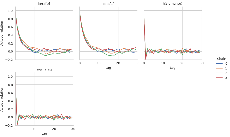
Finally, let’s check the autocorrelation of the samples.

gs.plot_cor(results)