Parameter transformations#
This tutorial builds on the linear regression tutorial. Here, we demonstrate how we can easily transform a parameter in our model to sample it with NUTS instead of a Gibbs Kernel.
First, let’s set up our model again. This is the same model as in the linear regression tutorial, so we will not go into the details here.
import jax
import jax.numpy as jnp
import liesel.goose as gs
import liesel.model as lsl
import matplotlib.pyplot as plt
import numpy as np

# We use distributions and bijectors from tensorflow probability
import tensorflow_probability.substrates.jax.distributions as tfd
import tensorflow_probability.substrates.jax.bijectors as tfb

rng = np.random.default_rng(42)

# data-generating process
n = 500
true_beta = np.array([1.0, 2.0])
true_sigma = 1.0
x0 = rng.uniform(size=n)
X_mat = np.column_stack([np.ones(n), x0])
eps = rng.normal(scale=true_sigma, size=n)
y_vec = X_mat @ true_beta + eps

# Model
# Part 1: Model for the mean
beta_loc = lsl.Var(0.0, name="beta_loc")
beta_scale = lsl.Var(100.0, name="beta_scale") # scale = sqrt(100^2)
beta_dist = lsl.Dist(tfd.Normal, loc=beta_loc, scale=beta_scale)
beta = lsl.Param(value=np.array([0.0, 0.0]), distribution=beta_dist,name="beta")

X = lsl.Obs(X_mat, name="X")
calc = lsl.Calc(lambda x, beta: jnp.dot(x, beta), x=X, beta=beta)
y_hat = lsl.Var(calc, name="y_hat")

# Part 2: Model for the standard deviation
sigma_a = lsl.Var(0.01, name="a")
sigma_b = lsl.Var(0.01, name="b")
sigma_dist = lsl.Dist(tfd.InverseGamma, concentration=sigma_a, scale=sigma_b)
sigma = lsl.Param(value=10.0, distribution=sigma_dist, name="sigma")

# Observation model
y_dist = lsl.Dist(tfd.Normal, loc=y_hat, scale=sigma)
y = lsl.Var(y_vec, distribution=y_dist, name="y")
Now let’s try to sample the full parameter vector
\((\boldsymbol{\beta}', \sigma)'\) with a single NUTS kernel instead of
using a NUTS kernel for \(\boldsymbol{\beta}\) and a Gibbs kernel for
\(\sigma\). Since the standard deviation is a positive-valued parameter,
we need to log-transform it to sample it with a NUTS kernel. The
GraphBuilder class provides the transform_parameter()
method for this purpose.
gb = lsl.GraphBuilder().add(y)
gb.transform(sigma, tfb.Exp)
Var<sigma_transformed>

No GPU/TPU found, falling back to CPU. (Set TF_CPP_MIN_LOG_LEVEL=0 and rerun for more info.)
model = gb.build_model()
lsl.plot_vars(model)
![]()
The response distribution still requires the standard deviation on the
original scale. The model graph shows that the back-transformation from
the logarithmic to the original scale is performed by a inserting the
sigma_transformed and turning the sigma node into a weak node. This
weak node deterministically depends on sigma_transformed: its value is
the back-transformed standard deviation.
Now we can set up and run an MCMC algorithm with a NUTS kernel for all parameters.
builder = gs.EngineBuilder(seed=1339, num_chains=4)

builder.set_model(lsl.GooseModel(model))
builder.set_initial_values(model.state)

builder.add_kernel(gs.NUTSKernel(["beta", "sigma_transformed"]))

builder.set_duration(warmup_duration=1000, posterior_duration=1000)

# by default, goose only stores the parameters specified in the kernels.
# let's also store the standard deviation on the original scale.
builder.positions_included = ["sigma"]

engine = builder.build()
engine.sample_all_epochs()
liesel.goose.engine - INFO - Starting epoch: FAST_ADAPTATION, 75 transitions, 25 jitted together
liesel.goose.engine - WARNING - Errors per chain for kernel_00: 2, 3, 2, 5 / 75 transitions
liesel.goose.engine - INFO - Finished epoch
liesel.goose.engine - INFO - Starting epoch: SLOW_ADAPTATION, 25 transitions, 25 jitted together
liesel.goose.engine - WARNING - Errors per chain for kernel_00: 1, 1, 1, 1 / 25 transitions
liesel.goose.engine - INFO - Finished epoch
liesel.goose.engine - INFO - Starting epoch: SLOW_ADAPTATION, 50 transitions, 25 jitted together
liesel.goose.engine - WARNING - Errors per chain for kernel_00: 2, 1, 1, 1 / 50 transitions
liesel.goose.engine - INFO - Finished epoch
liesel.goose.engine - INFO - Starting epoch: SLOW_ADAPTATION, 100 transitions, 25 jitted together
liesel.goose.engine - WARNING - Errors per chain for kernel_00: 2, 3, 2, 1 / 100 transitions
liesel.goose.engine - INFO - Finished epoch
liesel.goose.engine - INFO - Starting epoch: SLOW_ADAPTATION, 200 transitions, 25 jitted together
liesel.goose.engine - WARNING - Errors per chain for kernel_00: 1, 6, 4, 0 / 200 transitions
liesel.goose.engine - INFO - Finished epoch
liesel.goose.engine - INFO - Starting epoch: SLOW_ADAPTATION, 500 transitions, 25 jitted together
liesel.goose.engine - WARNING - Errors per chain for kernel_00: 1, 3, 3, 4 / 500 transitions
liesel.goose.engine - INFO - Finished epoch
liesel.goose.engine - INFO - Starting epoch: FAST_ADAPTATION, 50 transitions, 25 jitted together
liesel.goose.engine - WARNING - Errors per chain for kernel_00: 1, 3, 1, 1 / 50 transitions
liesel.goose.engine - INFO - Finished epoch
liesel.goose.engine - INFO - Finished warmup
liesel.goose.engine - INFO - Starting epoch: POSTERIOR, 1000 transitions, 25 jitted together
liesel.goose.engine - INFO - Finished epoch
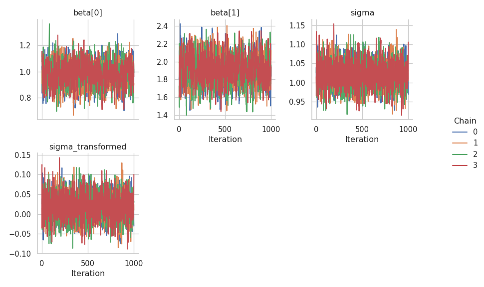
Judging from the trace plots, it seems that all chains have converged.
results = engine.get_results()
g = gs.plot_trace(results)
We can also take a look at the summary table, which includes the original \(\sigma\) and the transformed \(\log(\sigma)\).
gs.Summary.from_result(results)
Parameter summary:
| kernel | mean | sd | q_0.05 | q_0.5 | q_0.95 | sample_size | ess_bulk | ess_tail | rhat | ||
|---|---|---|---|---|---|---|---|---|---|---|---|
| parameter | index | ||||||||||
| beta | (0,) | kernel_00 | 0.985 | 0.092 | 0.831 | 0.988 | 1.133 | 4000 | 1347.289 | 1782.123 | 1.002 |
| (1,) | kernel_00 | 1.906 | 0.162 | 1.642 | 1.902 | 2.183 | 4000 | 1279.326 | 1637.940 | 1.003 | |
| sigma | () | \- | 1.021 | 0.033 | 0.967 | 1.021 | 1.077 | 4000 | 2517.353 | 2191.691 | 1.000 |
| sigma_transformed | () | kernel_00 | 0.020 | 0.033 | -0.033 | 0.021 | 0.074 | 4000 | 2517.356 | 2191.691 | 1.000 |
Error summary:
| count | relative | ||||
|---|---|---|---|---|---|
| kernel | error_code | error_msg | phase | ||
| kernel_00 | 1 | divergent transition | warmup | 57 | 0.014 |
| posterior | 0 | 0.000 |
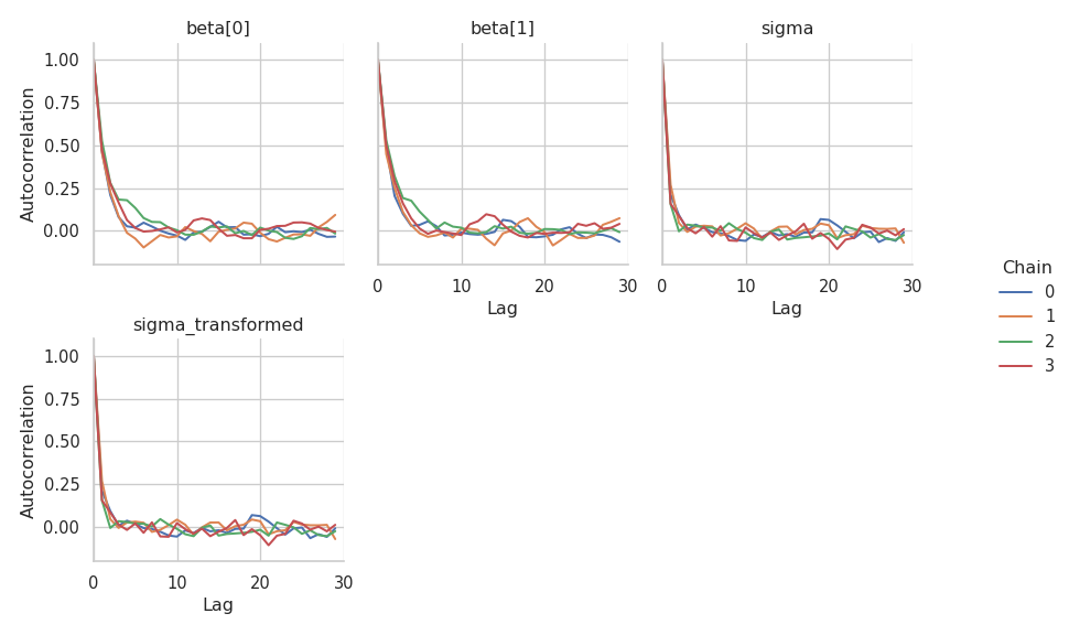
The effective sample size is higher for \(\sigma\) than for \(\boldsymbol{\beta}\). Finally, let’s check the autocorrelation of the samples.
g = gs.plot_cor(results)