GEV responses#
In this tutorial, we illustrate how to set up a distributional regression model with the generalized extreme value distribution as a response distribution. First, we simulate some data in R:
The location parameter (\(\mu\)) is a function of an intercept and a non-linear covariate effect.
The scale parameter (\(\sigma\)) is a function of an intercept and a linear effect and uses a log-link.
The shape or concentration parameter (\(\xi\)) is a function of an intercept and a linear effect.
After simulating the data, we can configure the model with a single call
to the rliesel::liesel() function.
library(rliesel)
Please set your Liesel venv, e.g. with use_liesel_venv()
library(VGAM)
Loading required package: stats4

Loading required package: splines
set.seed(1337)
n <- 1000
x0 <- runif(n)
x1 <- runif(n)
x2 <- runif(n)
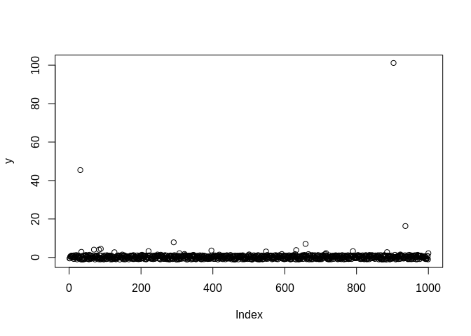
y <- rgev(
n,
location = 0 + sin(2 * pi * x0),
scale = exp(-3 + x1),
shape = 0.1 + x2
)
plot(y)
model <- liesel(
  response = y,
  distribution = "GeneralizedExtremeValue",
  predictors = list(
    loc = predictor(~ s(x0)),
    scale = predictor(~ x1, inverse_link = "Exp"),
    concentration = predictor(~ x2)
  )
)
Now, we can continue in Python and use the lsl.dist_reg_mcmc()
function to set up a sampling algorithm with IWLS kernels for the
regression coefficients (\(\boldsymbol{\beta}\)) and a Gibbs kernel for
the smoothing parameter (\(\tau^2\)) of the spline. Note that we need to
set \(\beta_0\) for \(\xi\) to 0.1 manually, because \(\xi = 0\) breaks the
sampler.
import liesel.model as lsl
import jax.numpy as jnp

model = r.model

# concentration == 0.0 seems to break the sampler
model.vars["concentration_p0_beta"].value = jnp.array([0.1, 0.0])

builder = lsl.dist_reg_mcmc(model, seed=42, num_chains=4)
builder.set_duration(warmup_duration=1000, posterior_duration=1000)

engine = builder.build()
engine.sample_all_epochs()
liesel.goose.engine - INFO - Starting epoch: FAST_ADAPTATION, 75 transitions, 25 jitted together
liesel.goose.engine - WARNING - Errors per chain for kernel_00: 8, 11, 5, 4 / 75 transitions
liesel.goose.engine - WARNING - Errors per chain for kernel_01: 0, 0, 1, 0 / 75 transitions
liesel.goose.engine - WARNING - Errors per chain for kernel_03: 1, 0, 0, 0 / 75 transitions
liesel.goose.engine - INFO - Finished epoch
liesel.goose.engine - INFO - Starting epoch: SLOW_ADAPTATION, 25 transitions, 25 jitted together
liesel.goose.engine - WARNING - Errors per chain for kernel_00: 0, 1, 2, 3 / 25 transitions
liesel.goose.engine - WARNING - Errors per chain for kernel_01: 1, 1, 1, 1 / 25 transitions
liesel.goose.engine - WARNING - Errors per chain for kernel_03: 1, 1, 1, 1 / 25 transitions
liesel.goose.engine - WARNING - Errors per chain for kernel_04: 2, 1, 3, 1 / 25 transitions
liesel.goose.engine - INFO - Finished epoch
liesel.goose.engine - INFO - Starting epoch: SLOW_ADAPTATION, 50 transitions, 25 jitted together
liesel.goose.engine - WARNING - Errors per chain for kernel_00: 3, 3, 2, 1 / 50 transitions
liesel.goose.engine - WARNING - Errors per chain for kernel_01: 0, 0, 1, 2 / 50 transitions
liesel.goose.engine - WARNING - Errors per chain for kernel_03: 2, 1, 1, 1 / 50 transitions
liesel.goose.engine - WARNING - Errors per chain for kernel_04: 1, 1, 1, 0 / 50 transitions
liesel.goose.engine - INFO - Finished epoch
liesel.goose.engine - INFO - Starting epoch: SLOW_ADAPTATION, 100 transitions, 25 jitted together
liesel.goose.engine - WARNING - Errors per chain for kernel_00: 2, 2, 2, 2 / 100 transitions
liesel.goose.engine - WARNING - Errors per chain for kernel_01: 1, 1, 3, 0 / 100 transitions
liesel.goose.engine - WARNING - Errors per chain for kernel_03: 1, 2, 1, 1 / 100 transitions
liesel.goose.engine - WARNING - Errors per chain for kernel_04: 0, 2, 2, 2 / 100 transitions
liesel.goose.engine - INFO - Finished epoch
liesel.goose.engine - INFO - Starting epoch: SLOW_ADAPTATION, 200 transitions, 25 jitted together
liesel.goose.engine - WARNING - Errors per chain for kernel_00: 3, 2, 1, 2 / 200 transitions
liesel.goose.engine - WARNING - Errors per chain for kernel_01: 1, 0, 2, 2 / 200 transitions
liesel.goose.engine - WARNING - Errors per chain for kernel_03: 2, 1, 1, 1 / 200 transitions
liesel.goose.engine - WARNING - Errors per chain for kernel_04: 1, 0, 2, 1 / 200 transitions
liesel.goose.engine - INFO - Finished epoch
liesel.goose.engine - INFO - Starting epoch: SLOW_ADAPTATION, 500 transitions, 25 jitted together
liesel.goose.engine - WARNING - Errors per chain for kernel_00: 2, 1, 3, 4 / 500 transitions
liesel.goose.engine - WARNING - Errors per chain for kernel_01: 1, 2, 1, 1 / 500 transitions
liesel.goose.engine - WARNING - Errors per chain for kernel_03: 1, 1, 1, 2 / 500 transitions
liesel.goose.engine - WARNING - Errors per chain for kernel_04: 1, 1, 3, 1 / 500 transitions
liesel.goose.engine - INFO - Finished epoch
liesel.goose.engine - INFO - Starting epoch: FAST_ADAPTATION, 50 transitions, 25 jitted together
liesel.goose.engine - WARNING - Errors per chain for kernel_00: 1, 3, 2, 1 / 50 transitions
liesel.goose.engine - WARNING - Errors per chain for kernel_01: 1, 1, 0, 0 / 50 transitions
liesel.goose.engine - WARNING - Errors per chain for kernel_03: 1, 1, 0, 1 / 50 transitions
liesel.goose.engine - WARNING - Errors per chain for kernel_04: 2, 1, 0, 2 / 50 transitions
liesel.goose.engine - INFO - Finished epoch
liesel.goose.engine - INFO - Finished warmup
liesel.goose.engine - INFO - Starting epoch: POSTERIOR, 1000 transitions, 25 jitted together
liesel.goose.engine - WARNING - Errors per chain for kernel_00: 0, 1, 4, 3 / 1000 transitions
liesel.goose.engine - INFO - Finished epoch
Some tabular summary statistics of the posterior samples:
import liesel.goose as gs

results = engine.get_results()
gs.Summary(results)
Parameter summary:
| kernel | mean | sd | q_0.05 | q_0.5 | q_0.95 | sample_size | ess_bulk | ess_tail | rhat | ||
|---|---|---|---|---|---|---|---|---|---|---|---|
| parameter | index | ||||||||||
| concentration_p0_beta | (0,) | kernel_00 | 0.069 | 0.050 | -0.011 | 0.069 | 0.152 | 4000 | 325.513 | 570.711 | 1.012 |
| (1,) | kernel_00 | 1.066 | 0.099 | 0.905 | 1.064 | 1.228 | 4000 | 146.567 | 557.704 | 1.024 | |
| loc_np0_beta | (0,) | kernel_03 | 0.600 | 0.225 | 0.231 | 0.599 | 0.966 | 4000 | 46.596 | 98.020 | 1.080 |
| (1,) | kernel_03 | 0.323 | 0.124 | 0.113 | 0.324 | 0.523 | 4000 | 99.516 | 251.131 | 1.054 | |
| (2,) | kernel_03 | -0.366 | 0.128 | -0.617 | -0.354 | -0.177 | 4000 | 45.433 | 70.262 | 1.083 | |
| (3,) | kernel_03 | 0.362 | 0.066 | 0.248 | 0.364 | 0.473 | 4000 | 63.030 | 151.633 | 1.054 | |
| (4,) | kernel_03 | -0.244 | 0.086 | -0.386 | -0.244 | -0.098 | 4000 | 63.526 | 156.110 | 1.089 | |
| (5,) | kernel_03 | 0.170 | 0.031 | 0.120 | 0.169 | 0.222 | 4000 | 53.459 | 132.167 | 1.097 | |
| (6,) | kernel_03 | 6.027 | 0.037 | 5.970 | 6.025 | 6.091 | 4000 | 74.895 | 249.095 | 1.032 | |
| (7,) | kernel_03 | 0.545 | 0.072 | 0.428 | 0.546 | 0.662 | 4000 | 49.211 | 178.115 | 1.106 | |
| (8,) | kernel_03 | 1.702 | 0.029 | 1.656 | 1.701 | 1.751 | 4000 | 70.823 | 211.549 | 1.034 | |
| loc_np0_tau2 | () | kernel_02 | 6.286 | 5.865 | 2.419 | 5.091 | 13.444 | 4000 | 3625.394 | 3754.696 | 1.000 |
| loc_p0_beta | (0,) | kernel_04 | 0.027 | 0.003 | 0.023 | 0.027 | 0.032 | 4000 | 81.008 | 81.954 | 1.050 |
| scale_p0_beta | (0,) | kernel_01 | -3.063 | 0.060 | -3.159 | -3.064 | -2.962 | 4000 | 84.917 | 151.014 | 1.037 |
| (1,) | kernel_01 | 1.040 | 0.076 | 0.914 | 1.040 | 1.166 | 4000 | 150.826 | 360.761 | 1.014 |
Error summary:
| count | relative | ||||
|---|---|---|---|---|---|
| kernel | error_code | error_msg | phase | ||
| kernel_00 | 90 | nan acceptance prob | warmup | 76 | 0.019 |
| posterior | 8 | 0.002 | |||
| kernel_01 | 90 | nan acceptance prob | warmup | 25 | 0.006 |
| posterior | 0 | 0.000 | |||
| kernel_03 | 90 | nan acceptance prob | warmup | 28 | 0.007 |
| posterior | 0 | 0.000 | |||
| kernel_04 | 90 | nan acceptance prob | warmup | 31 | 0.008 |
| posterior | 0 | 0.000 |
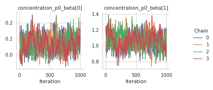
And the corresponding trace plots:
fig = gs.plot_trace(results, "loc_p0_beta")
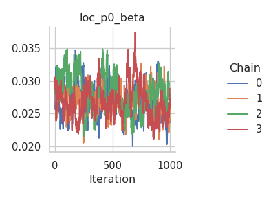
fig = gs.plot_trace(results, "loc_np0_tau2")
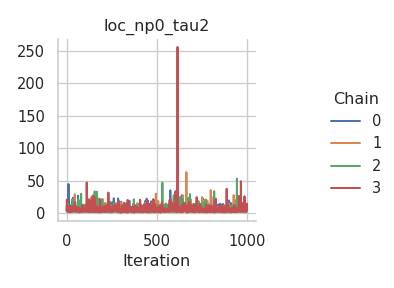
fig = gs.plot_trace(results, "loc_np0_beta")
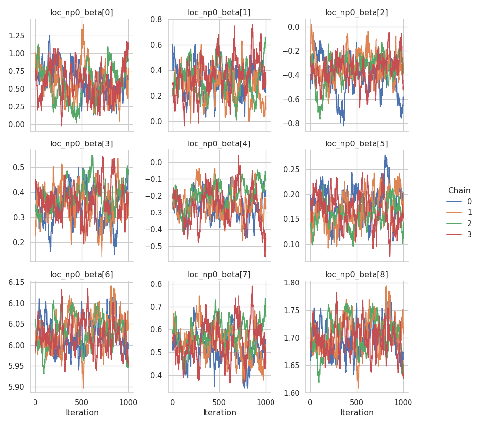
fig = gs.plot_trace(results, "scale_p0_beta")
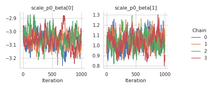
fig = gs.plot_trace(results, "concentration_p0_beta")
We need to reset the index of the summary data frame before we can transfer it to R.
summary = gs.Summary(results).to_dataframe().reset_index()
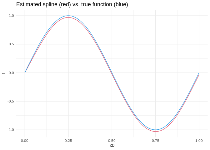
After transferring the summary data frame to R, we can process it with packages like dplyr and ggplot2. Here is a visualization of the estimated spline vs. the true function:
library(dplyr)
Attaching package: 'dplyr'

The following objects are masked from 'package:stats':

    filter, lag

The following objects are masked from 'package:base':

    intersect, setdiff, setequal, union
library(ggplot2)
library(reticulate)

summary <- py$summary

beta <- summary %>%
  filter(variable == "loc_np0_beta") %>%
  group_by(var_index) %>%
  summarize(mean = mean(mean)) %>%
  ungroup()

beta <- beta$mean
X <- py_to_r(model$vars["loc_np0_X"]$value)
estimate <- X %*% beta

true <- sin(2 * pi * x0)

ggplot(data.frame(x0 = x0, estimate = estimate, true = true)) +
  geom_line(aes(x0, estimate), color = palette()[2]) +
  geom_line(aes(x0, true), color = palette()[4]) +
  ggtitle("Estimated spline (red) vs. true function (blue)") +
  ylab("f") +
  theme_minimal()