PyMC and Liesel: Spike and Slab#

Liesel provides an interface for PyMC, a popular Python library for Bayesian Models. In this tutorial, we see how to specify a model in PyMC and then fit it using Liesel.

Be sure that you have pymc installed. If that’s not the case, you can install Liesel with the optional dependency PyMC.

pip install liesel[pymc]

We will build a Spike and Slab model, a Bayesian approach that allows for variable selection by assuming a mixture of two distributions for the prior distribution of the regression coefficients: a point mass at zero (the “spike”) and a continuous distribution centered around zero (the “slab”). The model assumes that each coefficient \(\beta_j\) has a corresponding indicator variable \(\delta_j\) that takes a value of either 0 or 1, indicating whether the variable is included in the model or not. The prior distribution of the indicator variables is a Bernoulli distribution, with a parameter \(\theta\) that controls the sparsity of the model. When the parameter is close to 1, the model is more likely to include all variables, while when it is close to 0, the model is more likely to select only a few variables. In our case, we assign a Beta hyperprior to \(\theta\):

\[\begin{split} \begin{eqnarray} \mathbf{y} &\sim& \mathcal{N} \left( \mathbf{X}\boldsymbol{\beta}, \sigma^2 \mathbf{I} \right)\\ \boldsymbol{\beta}_j &\sim& \mathbfcal{N}\left(0, (1 - \delta_j)\nu + \delta_j\tau^2_j / \sigma^2 \right)\\ \tau^2_j &\sim& \mathcal{IG}(\text{a}_{\tau}, \text{b}_{\tau})\\ \delta_j &\sim& \text{Bernoulli}(\theta)\\ \theta &\sim& \text{Beta}(\text{a}_\theta, \text{b}_\theta)\\ \sigma^2 &\sim& \mathcal{IG}(\text{a}_{\sigma^2}, \text{b}_{\sigma^2}) \end{eqnarray}. \end{split}\]

where \(\nu\) is a hyperparameter that we set to a fixed small value. That way, when \(\delta_j = 0\), the prior variance for \(\beta_j\) is extremely small, practically forcing it to be close to zero.

First, we generate the data. We use a model with four coefficients but assume that only two variables are relevant, namely the first and the third one.

RANDOM_SEED = 123
rng = np.random.RandomState(RANDOM_SEED)

n = 1000
p = 4

sigma_scalar = 1.0
beta_vec = np.array([3.0, 0.0, 4.0, 0.0])

X = rng.randn(n, p).astype(np.float32)

errors = rng.normal(size=n).astype(np.float32)

y = X @ beta_vec + sigma_scalar * errors

Then, we can specify the model using PyMC.

spike_and_slab_model = pm.Model()

mu = 0.

alpha_tau = 1.0
beta_tau = 1.0

alpha_sigma = 1.0
beta_sigma = 1.0

alpha_theta = 8.0
beta_theta = 8.0

nu = 0.1

with spike_and_slab_model:
    # priors
    sigma2 = pm.InverseGamma(
        "sigma2", alpha=alpha_sigma, beta=beta_sigma
    )

    theta = pm.Beta("theta", alpha=alpha_theta, beta=beta_theta)
    delta = pm.Bernoulli("delta", p=theta, size=p)
    tau = pm.InverseGamma("tau", alpha=alpha_tau, beta=beta_tau)

    beta = pm.Normal("beta", mu=0.0, sigma=nu * (1 - delta) + delta * pm.math.sqrt(tau / sigma2), shape=p)

    # likelihood
    pm.Normal("y", mu=X @ beta, sigma=pm.math.sqrt(sigma2), observed=y)

Let’s take a look at our model:

spike_and_slab_model

<pymc.model.Model object at 0x7fae106656c0>

The class PyMCInterface offers an interface between PyMC and Goose. By default, the constructor of PyMCInterface keeps track only of a representation of random variables that can be used in sampling. For example, theta is transformed to the real-numbers space with a log-odds transformation, and therefore the model only keeps track of theta_log_odds__. However, we would like to access the untransformed samples as well. We can do this by including them in the additional_vars argument of the constructor of the interface.

The initial position can be extracted with get_initial_state(). The model state is represented as a Position.

interface = PyMCInterface(spike_and_slab_model, additional_vars=["sigma2", "tau", "theta"])

No GPU/TPU found, falling back to CPU. (Set TF_CPP_MIN_LOG_LEVEL=0 and rerun for more info.)

state = interface.get_initial_state()

Since \(\delta_j\) is a discrete variable, we need to use a Gibbs sampler to draw samples for it. Unfortunately, we cannot derive the posterior analytically, but what we can do is use a Metropolis-Hastings step as a transition function:

def delta_transition_fn(prng_key, model_state):
    draw_key, mh_key = jax.random.split(prng_key)
    theta_logodds = model_state["theta_logodds__"]
    p = jax.numpy.exp(theta_logodds) / (1 + jax.numpy.exp(theta_logodds))
    draw = jax.random.bernoulli(draw_key, p=p, shape=(4,))
    proposal = {"delta": jax.numpy.asarray(draw,dtype=np.int64)}
    _, state = gs.mh.mh_step(prng_key=mh_key, model=interface, proposal=proposal, model_state=model_state)
    return state

Finally, we can sample from the posterior as we do for any other Liesel model. In this case, we use a GibbsKernel for \(\boldsymbol{\delta}\) and a NUTSKernel both for the remaining parameters.

builder = gs.EngineBuilder(seed=13, num_chains=4)
builder.set_model(interface)
builder.set_initial_values(state)
builder.set_duration(warmup_duration=1000, posterior_duration=2000)

builder.add_kernel(gs.NUTSKernel(position_keys=["beta", "sigma2_log__", "tau_log__", "theta_logodds__"]))
builder.add_kernel(gs.GibbsKernel(["delta"], transition_fn=delta_transition_fn))

builder.positions_included = ["sigma2", "tau"]

engine = builder.build()

/opt/hostedtoolcache/Python/3.10.10/x64/lib/python3.10/site-packages/pytensor/link/jax/dispatch/elemwise.py:35: UserWarning: Explicitly requested dtype float64 requested in astype is not available, and will be truncated to dtype float32. To enable more dtypes, set the jax_enable_x64 configuration option or the JAX_ENABLE_X64 shell environment variable. See https://github.com/google/jax#current-gotchas for more.
  return jax_op(x, axis=axis).astype(acc_dtype)

engine.sample_all_epochs()

liesel.goose.engine - INFO - Starting epoch: FAST_ADAPTATION, 75 transitions, 25 jitted together
<string>:6: UserWarning: Explicitly requested dtype <class 'numpy.int64'> requested in asarray is not available, and will be truncated to dtype int32. To enable more dtypes, set the jax_enable_x64 configuration option or the JAX_ENABLE_X64 shell environment variable. See https://github.com/google/jax#current-gotchas for more.
liesel.goose.engine - WARNING - Errors per chain for kernel_00: 2, 2, 2, 3 / 75 transitions
liesel.goose.engine - INFO - Finished epoch
liesel.goose.engine - INFO - Starting epoch: SLOW_ADAPTATION, 25 transitions, 25 jitted together
liesel.goose.engine - WARNING - Errors per chain for kernel_00: 1, 1, 1, 1 / 25 transitions
liesel.goose.engine - INFO - Finished epoch
liesel.goose.engine - INFO - Starting epoch: SLOW_ADAPTATION, 50 transitions, 25 jitted together
liesel.goose.engine - WARNING - Errors per chain for kernel_00: 0, 0, 0, 1 / 50 transitions
liesel.goose.engine - INFO - Finished epoch
liesel.goose.engine - INFO - Starting epoch: SLOW_ADAPTATION, 100 transitions, 25 jitted together
liesel.goose.engine - WARNING - Errors per chain for kernel_00: 1, 1, 2, 1 / 100 transitions
liesel.goose.engine - INFO - Finished epoch
liesel.goose.engine - INFO - Starting epoch: SLOW_ADAPTATION, 200 transitions, 25 jitted together
liesel.goose.engine - WARNING - Errors per chain for kernel_00: 1, 1, 1, 1 / 200 transitions
liesel.goose.engine - INFO - Finished epoch
liesel.goose.engine - INFO - Starting epoch: SLOW_ADAPTATION, 500 transitions, 25 jitted together
liesel.goose.engine - WARNING - Errors per chain for kernel_00: 1, 1, 1, 1 / 500 transitions
liesel.goose.engine - INFO - Finished epoch
liesel.goose.engine - INFO - Starting epoch: FAST_ADAPTATION, 50 transitions, 25 jitted together
liesel.goose.engine - WARNING - Errors per chain for kernel_00: 1, 1, 2, 1 / 50 transitions
liesel.goose.engine - INFO - Finished epoch
liesel.goose.engine - INFO - Finished warmup
liesel.goose.engine - INFO - Starting epoch: POSTERIOR, 2000 transitions, 25 jitted together
liesel.goose.engine - INFO - Finished epoch

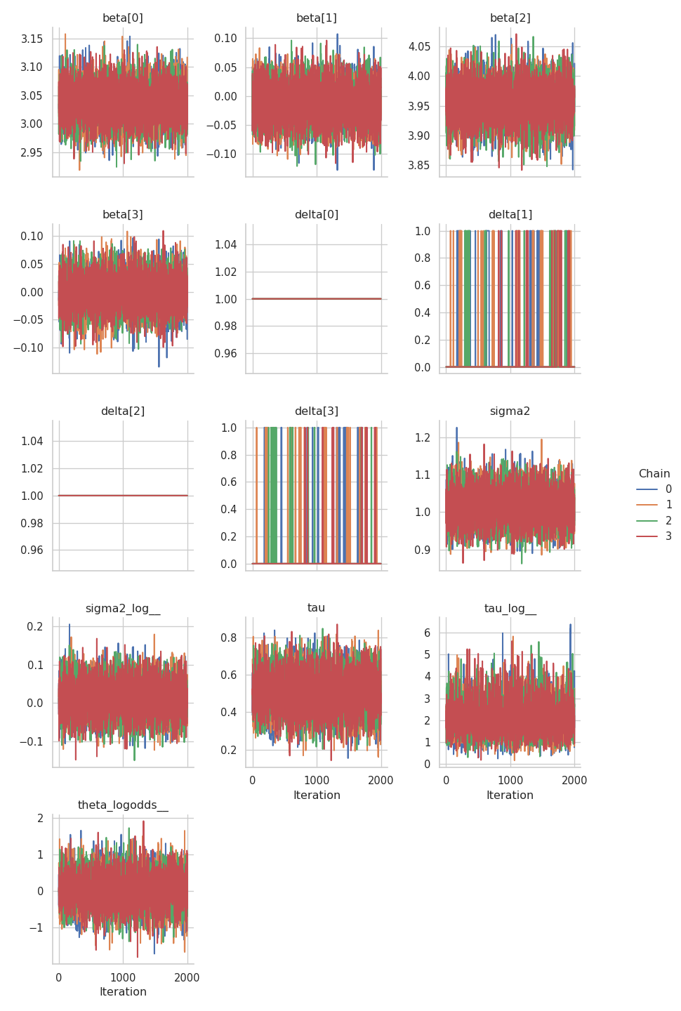
Now, we can take a look at the summary of the results and at the trace plots.

results = engine.get_results()
print(gs.Summary(results))

                         var_fqn     kernel  ...   hdi_low  hdi_high
variable                                     ...                    
beta                     beta[0]  kernel_00  ...  2.985217  3.088682
beta                     beta[1]  kernel_00  ... -0.061793  0.039922
beta                     beta[2]  kernel_00  ...  3.904587  4.007628
beta                     beta[3]  kernel_00  ... -0.053403  0.046218
delta                   delta[0]  kernel_01  ...  1.000000  1.000000
delta                   delta[1]  kernel_01  ...  0.000000  0.000000
delta                   delta[2]  kernel_01  ...  1.000000  1.000000
delta                   delta[3]  kernel_01  ...  0.000000  0.000000
sigma2                    sigma2          -  ...  0.939147  1.086152
sigma2_log__        sigma2_log__  kernel_00  ... -0.061589  0.083753
tau                          tau          -  ...  0.318184  0.678991
tau_log__              tau_log__  kernel_00  ...  0.908542  3.308814
theta_logodds__  theta_logodds__  kernel_00  ... -0.762132  0.749137

[13 rows x 17 columns]

/opt/hostedtoolcache/Python/3.10.10/x64/lib/python3.10/site-packages/arviz/stats/diagnostics.py:592: RuntimeWarning: invalid value encountered in scalar divide
  (between_chain_variance / within_chain_variance + num_samples - 1) / (num_samples)

As we can see from the posterior means of the \(\boldsymbol{\delta}\) parameters, the model was able to recognize those variable with no influence on the respose \(\mathbf{y}\):

\(\delta_1\) and \(\delta_3\) (delta[0] and delta[2] in the table) have a posterior mean of \(1\), indicating inclusion.
\(\delta_2\) and \(\delta_4\) (delta[1] and delta[3] in the table) have a posterior mean of \(0.06\), indicating exclusion.

gs.plot_trace(results)