Advanced Group Usage#

This is a tutorial on how Liesel’s Group class can be used to derive new classes that represent re-usable model parts. This tutorial covers the following parts:

Derive new classes from Group to represent related Vars.
Use these groups to create a Gibbs kernel.

Background#

As the topic for this group tutorial, we will create groups for a semiparametric regression model using Bayesian P-Splines. In this tutorial, we only give minimal background on the model itself - instead, for details on the model, the interested reader should consider the original paper by Lang & Brezger (2012).

In Bayesian P-Splines, we try to estimate a function \(f(x)\) of a covariate \(x\) - which may, for example represented the relationship between \(x\) and the response’s mean. To implement the estination, we parameterize the functione estimate by the product of a design matrix of basis function evaluations \(\boldsymbol{B}(x)\) and a vector of spline coefficients \(\boldsymbol{\beta}\), i.e. \(f(x) \approx \boldsymbol{B}(x)\boldsymbol{\beta}\). The goal is to estimate \(\boldsymbol{\beta}\). In Bayesian P-Splines, we are commonly working with a rank-deficient (degenerate) multivariate normal prior on \(\boldsymbol{\beta}\). The unnormalized prior can be written as

\[ p(\boldsymbol{\beta}) \propto \exp\left( - \frac{1}{2\tau^2} \boldsymbol{\beta}^T \boldsymbol{K} \boldsymbol{\beta} \right), \]

where \(\boldsymbol{K}\) is an appropriately defined penalty matrix, commonly a rank-deficient squared second order difference matrix where the variance and the parameter \(\tau^2\) controls the amount of strength of the penalty (usually a large \(\tau^2\) allows for a wiggly function) and corresponds to an inverse smoothing parameter.

In Bayesian P-Splines, the variance parameter \(\tau^2\) receives a hyperprior. A common choice is to set

\[ \tau^2 \sim \text{InverseGamma}(a, b) \]

with shape \(a\) and scale \(b\) as hyperparameters. We will create one group each for \(\tau^2\) and for \(\boldsymbol{\beta}\). Then, we will create an overarching group that represents a complete P-Spline.

Setup#

We start by importing the modules that we are going to use in this tutorial.

import numpy as np
import jax.numpy as jnp
import jax
import tensorflow_probability.substrates.jax.distributions as tfd

import liesel.model as lsl
import liesel.goose as gs
from liesel.distributions.mvn_degen import MultivariateNormalDegenerate
from liesel.goose.types import Array

Define groups#

Inverse smoothing parameter \(\tau^2\)#

This is straight-forward group: We initialize it with a name, values for the hyperparameters of the inverse gamma prior, and an initial value for \(\tau^2\).

To do so, we simply overload the __init__ method, use this method to create the needed Vars and finalize initialization by calling the __init__ of the parent class. This last step makes sure that the individual nodes are correctly informed about their group membership.

Note that we use the group name here as the prefix the for names of the individual variables inside the group. That makes it easy to make these names unique within a model, which is a requirement for Liesel.

class VarianceIG(lsl.Group):
    def __init__(
        self, name: str, a: float, b: float, start_value: float = 1000.0
    ) -> None:
        a_var = lsl.Var(a, name=f"{name}_a")
        b_var = lsl.Var(b, name=f"{name}_b")

        prior = lsl.Dist(tfd.InverseGamma, concentration=a_var, scale=b_var)
        tau2 = lsl.Param(start_value, distribution=prior, name=name)
        super().__init__(name=name, a=a_var, b=b_var, tau2=tau2)

Spline coefficient#

Next, we create the group for our spline coefficient in a very similar way.

class SplineCoef(lsl.Group):
    def __init__(self, name: str, penalty: Array, tau2: lsl.Param) -> None:
        penalty_var = lsl.Var(penalty, name=f"{name}_penalty")

        # we save the rank of the penalty matrix here to use it later in our
        # gibbs kernel
        rank = lsl.Data(np.linalg.matrix_rank(penalty), _name=f"{name}_rank")

        prior = lsl.Dist(
            MultivariateNormalDegenerate.from_penalty,
            loc=0.0,
            var=tau2,
            pen=penalty_var,
        )
        start_value = np.zeros(np.shape(penalty)[-1], np.float32)

        coef = lsl.Param(start_value, distribution=prior, name=name)

        super().__init__(name, coef=coef, penalty=penalty_var, tau2=tau2, rank=rank)

Use groups#

We can use these groups to quickly create model building blocks and access their elements:

tau2_group = VarianceIG(name="tau2", a=0.01, b=0.01)

print(tau2_group["tau2"])

Var(name="tau2")

We can directly use the tau2_group to create an instance of SplineCoef:

second_diff = np.diff(np.eye(10), n=2, axis=0)
penalty = second_diff.T @ second_diff
coef_group = SplineCoef(name="coef", penalty=penalty, tau2=tau2_group["tau2"])

Each group offers access to all its members through mappingproxy instances, which are basically immutable dictionaries:

tau2_group.vars

mappingproxy({'a': Var(name="tau2_a"), 'b': Var(name="tau2_b"), 'tau2': Var(name="tau2")})

coef_group.vars

mappingproxy({'coef': Var(name="coef"), 'penalty': Var(name="coef_penalty"), 'tau2': Var(name="tau2")})

A complete P-Spline group#

In this last step, we create an overarching group that incorporates the observed basis matrix of our spline and evaluates the estimated function \(\hat{f}(x) = \boldsymbol{B}(x)\hat{\boldsymbol{\beta}}\). Note the following:

Here, we create a SplineCoef instance inside the new group’s __init__, because this step is always the same with P-Splines, once we know the penalty and the variance parameter \(\tau^2\).
We do not automatically create an instance of our IGVariance group for the variance parameter, but allow users to pass any fitting group instance to the class. This makes our PSpline class very flexible: we could easily replace the IGVariance group with another group that represents a different prior for \(\tau^2\). For this PSpline group, it is only important that there is a key "tau2" in the tau2_group.
In the code below, we represent \(\hat{f}(x)\) with a variable named smooth to stay consistent with the terminology used in DistRegBuilder.
In our super().__init__ call at the end, we make sure to add not only the Vars basis_matrix and smooth that we directly created, but also all members of the coef_group and tau2_group. That way, we can access all relevant vars just from this overarching PSpline group.

class PSpline(lsl.Group):
    def __init__(
        self, name, basis_matrix: Array, penalty: Array, tau2_group: lsl.Group
    ) -> None:
        coef_group = SplineCoef(
            name=f"{name}_coef", penalty=penalty, tau2=tau2_group["tau2"]
        )

        basis_matrix = lsl.Obs(basis_matrix, name="basis_matrix")
        smooth = lsl.Var(
            lsl.Calc(jnp.dot, basis_matrix, coef_group["coef"]), name=name
        )

        group_vars = coef_group.nodes_and_vars | tau2_group.nodes_and_vars

        super().__init__(
            name=name,
            basis_matrix=basis_matrix,
            smooth=smooth,
            **group_vars
        )

Of course it may be convenient to specialize this PSpline group, depending on your usage. For example, we could imagine to adapt it to an IGPSpline group that works on the assumption that you want to use an inverse gamma prior on \(\tau^2\). Such a group would require the input parameters a and b instead of the tau2_group. The latter would be created automatically, just as the coef_group is in the code snippet above.

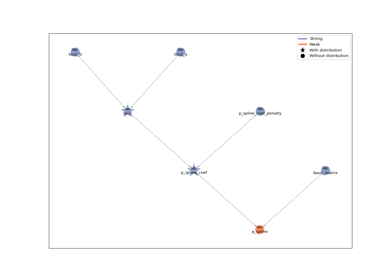
Group graph#

To see what we have created, let’s initialize a toy example of our group to look at the resulting graph. First, we create the group:

basis_matrix = np.random.uniform(size=(15, 10)) # NOT a valid basis matrix, just for show!

second_diff = np.diff(np.eye(10), n=2, axis=0)
penalty = second_diff.T @ second_diff

tau2_group = VarianceIG(name="tau2", a=0.01, b=0.01)
p_spline = PSpline(name="p_spline", basis_matrix=basis_matrix, penalty=penalty, tau2_group=tau2_group)

Next, we add this group to a GraphBuilder, build a model and plot the graph:

model = lsl.GraphBuilder().add_groups(p_spline).build_model()

liesel.model.model - INFO - Converted dtype of Data(name="p_spline_coef_penalty_value").value
liesel.model.model - INFO - Converted dtype of Data(name="basis_matrix_value").value
No GPU/TPU found, falling back to CPU. (Set TF_CPP_MIN_LOG_LEVEL=0 and rerun for more info.)

lsl.plot_vars(model)

Use group to build a Gibbs sampler#

When we use an inverse gamma prior for \(\tau^2\), we can set up a Gibbs sampler to sample from the posterior distribution of \(\tau^2\). In Liesel, we can conveniently define a GibbsKernel simply by supplying a stateless transition function and the name of the corresponding variable. Groups can help us to make this process modular, because they provide an interface with reliable and human-readable names for our variables.

What we actually want to do is to create a factory-function that takes our PSpline group as the input, creates an appropriate transition function under the hood and finally returns a fully functioning GibbsKernel.

def tau2_gibbs_kernel(p_spline: PSpline) -> gs.GibbsKernel:
    """Builds a Gibbs kernel for a smoothing parameter with an inverse gamma prior."""
    position_key = p_spline["tau2"].name

    def transition(prng_key, model_state):
        a_prior = p_spline.value_from(model_state, "a")
        b_prior = p_spline.value_from(model_state, "b")

        rank = p_spline.value_from(model_state, "rank")
        K = p_spline.value_from(model_state, "penalty")

        beta = p_spline.value_from(model_state, "coef")

        a_gibbs = jnp.squeeze(a_prior + 0.5 * rank)
        b_gibbs = jnp.squeeze(b_prior + 0.5 * (beta @ K @ beta))

        draw = b_gibbs / jax.random.gamma(prng_key, a_gibbs)

        return {position_key: draw}

    return gs.GibbsKernel([position_key], transition)

Most of the work here is done by the Group.value_from() method, which is nothing more than syntactic sugar for extracting a variable’s value from a model state using only the short and meaningful name of that variable within its group. For example, the call

beta = p_spline.value_from(model_state, "coef")

replaces a call like the following:

beta = model_state["long_unique_variable_name_coef"]

Supercharging your groups#

Groups are convenient tools for building re-usable model components. But with two simple tricks, they can be even more powerful:

Assign group members as attributes to the group. This enables syntax completion - do I need to say more?
Document the group’s init parameters and attributes. This will make your code much more re-usable by your future self and maybe even by other users.

Let’s consider an example using our IGVariance class from above:

class VarianceIG(lsl.Group):
    """
    Variance parameter with an inverse gamma prior.

    Parameters
    ----------
    name
        Group name. Will also be used as the name for the variance parameter variable.
    a
        Prior shape.
    b
        Prior scale.
    """
    def __init__(
        self, name: str, a: float, b: float, start_value: float = 1000.0
    ) -> None:
        self.a = lsl.Var(a, name="f{name}_a")
        """Prior shape variable."""

        self.b = lsl.Var(b, name="f{name}_b")
        """Prior scale variable."""

        prior = lsl.Dist(tfd.InverseGamma, concentration=a_var, scale=b_var)
        self.tau2 = lsl.Param(start_value, distribution=prior, name=name)
        """Variance parameter variable."""

        super().__init__(name=name, a=self.a, b=self.b, tau2=self.tau2)

This concludes our tutorial on group usage.

Advanced Group Usage

Contents