Location-scale regression#

This tutorial implements a Bayesian location-scale regression model within the Liesel framework. In contrast to the standard linear model with constant variance, the location-scale model allows for heteroscedasticity such that both the mean of the response variable as well as its variance depend on (possibly) different covariates.

This tutorial assumes a linear relationship between the expected value of the response and the regressors, whereas a logarithmic link is chosen for the standard deviation. More specifically, we choose the model

\[ \begin{aligned} y_i \sim \mathcal{N}_{} \left( \mathbf{x}_i^T \boldsymbol{\beta}, \exp \left( \mathbf{ z}_i^T \boldsymbol{\gamma} \right)^2 \right) \end{aligned} \]

in which the single observation are conditionally independent.

From the equation we see that location covariates are collected in the design matrix \(\mathbf{X}\) and scale covariates are contained in the design matrix \(\mathbf{ Z}\). Both matrices can, but generally do not have to, share common regressors. We refer to \(\boldsymbol{\beta}\) as location parameter and to \(\boldsymbol{\gamma}\) as scale parameter.

In this notebook, both design matrices only contain one intercept and one regressor column. However, the model design naturally generalizes to any (reasonable) number of covariates.

import jax
import jax.numpy as jnp
import liesel.goose as gs
import liesel.model as lsl
import matplotlib.pyplot as plt
import seaborn as sns
import tensorflow_probability.substrates.jax.distributions as tfd

sns.set_theme(style="whitegrid")

First lets generate the data according to the model

key = jax.random.PRNGKey(13)

No GPU/TPU found, falling back to CPU. (Set TF_CPP_MIN_LOG_LEVEL=0 and rerun for more info.)

n = 500

key, key_X, key_Z = jax.random.split(key, 3)

true_beta = jnp.array([1.0, 3.0])
true_gamma = jnp.array([0.0, 0.5])

X_mat = jnp.column_stack([jnp.ones(n), tfd.Uniform(low=0., high=5.).sample(n, seed=key_X)])
Z_mat = jnp.column_stack([jnp.ones(n), tfd.Normal(loc=2., scale=1.).sample(n, seed=key_Z)])

y_vec = jnp.zeros(n)
key_y = jax.random.split(key, n)

y_vec = jax.vmap(
    lambda x, beta, z, gamma, key: tfd.Normal(loc=x @ beta, scale=jnp.exp(z @ gamma)).sample(seed=key),
    (0, None, 0, None, 0))(X_mat, true_beta, Z_mat, true_gamma, key_y)

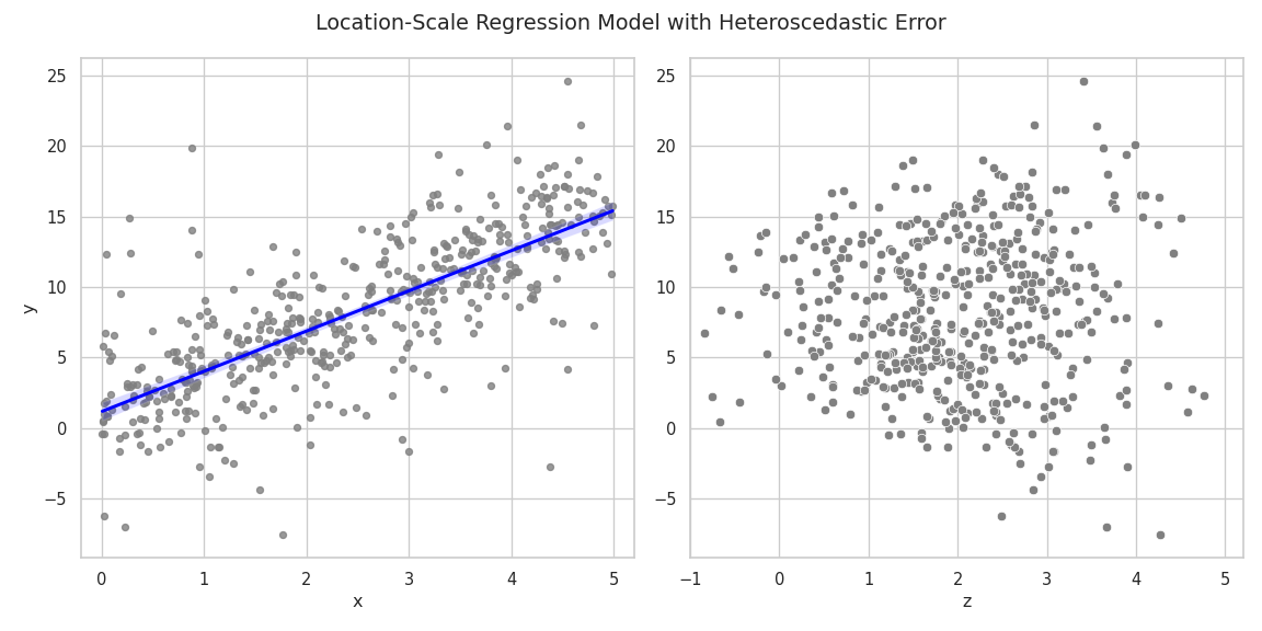
The simulated data displays a linear relationship between the response \(\mathbf{y}\) and the covariate \(\mathbf{x}\). The slope of the estimated regression line is close to the true \(\beta_1 = 3\). The right plot shows the relationship between \(\mathbf{y}\) and the scale covariate vector \(\mathbf{z}\). Larger values of \(\mathbf{ z}\) lead to a larger variance of the response.

fig, (ax1, ax2) = plt.subplots(nrows=1, ncols=2, figsize=(12, 6))
sns.regplot(
    x=X_mat[:, 1],
    y=y_vec,
    fit_reg=True,
    scatter_kws=dict(color="grey", s=20),
    line_kws=dict(color="blue"),
    ax=ax1,
).set(xlabel="x", ylabel="y", xlim=[-0.2, 5.2])

sns.scatterplot(
    x=Z_mat[:, 1],
    y=y_vec,
    color="grey",
    s=40,
    ax=ax2,
).set(xlabel="z", xlim=[-1, 5.2])

fig.suptitle("Location-Scale Regression Model with Heteroscedastic Error")
fig.tight_layout()
plt.show()

Since positivity of the variance is ensured by the exponential function, the linear part \(\mathbf{z}_i^T \boldsymbol{\gamma}\) is not restricted to the positive real line. Hence, setting a normal prior distribution for \(\gamma\) is feasible, leading to an almost symmetric specification of the location and scale parts of the model. The variables beta and gamma are initialized with values far away from zero to support a stable sampling process:

beta_loc = lsl.Var(0.0, name="beta_loc")
beta_scale = lsl.Var(100.0, name="beta_scale")

dist_beta = lsl.Dist(
    distribution=tfd.Normal, loc=beta_loc, scale=beta_scale
)
dist_beta = lsl.Dist(tfd.Normal, loc=beta_loc, scale=beta_scale)

beta = lsl.Param(
    value=jnp.array([10., 10.]), distribution=dist_beta, name="beta"
)

gamma_loc = lsl.Var(0.0, name="gamma_loc")
gamma_scale = lsl.Var(3.0, name="gamma_scale")

dist_gamma = lsl.Dist(
    distribution=tfd.Normal, loc=gamma_loc, scale=gamma_scale
)
gamma = lsl.Param(
    value=jnp.array([5.0, 5.0]), distribution=dist_gamma, name="gamma"
)

The additional complexity of the location-scale model compared to the standard linear model is handled in the next step. Since gamma takes values on the whole real line, but the response variable y expects a positive scale input, we need to apply the exponential function to the linear predictor to ensure positivity.

X = lsl.Obs(value=X_mat, name="X")
Z = lsl.Obs(value=Z_mat, name="Z")

mu = lsl.Var(lsl.Calc(lambda X, beta: X @ beta, X, beta), name="mu")
scale = lsl.Var(lsl.Calc(lambda Z, gamma: jnp.exp(Z @ gamma), Z, gamma), name="scale")

dist_y = lsl.Dist(distribution=tfd.Normal, loc=mu, scale=scale)
y = lsl.Obs(value=y_vec, distribution=dist_y, name="y")

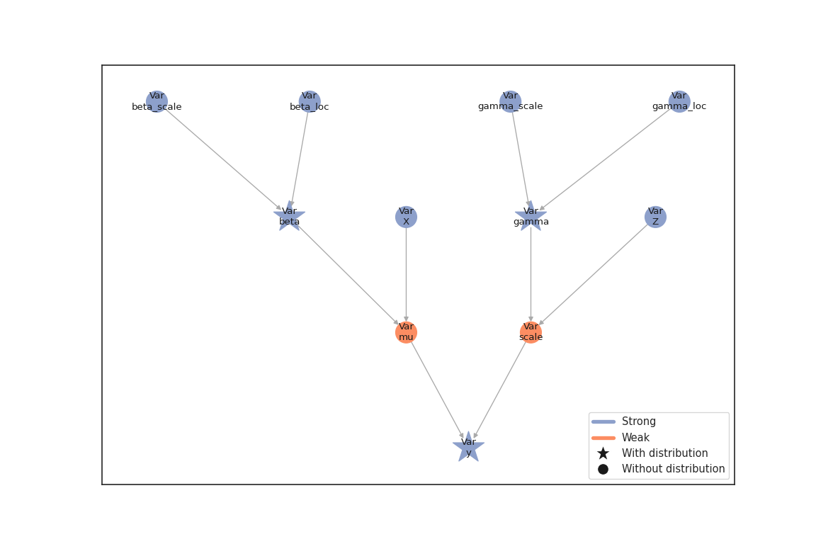
We can now combine the nodes in a model and visualize it

sns.set_theme(style="white")

gb = lsl.GraphBuilder()
gb.add(y)

GraphBuilder(0 nodes, 1 vars)

model = gb.build_model() # builds the model from the graph (PGMs)

lsl.plot_vars(model=model, width=12, height=8)

We choose the No U-Turn sampler for generating posterior samples. Therefore the location and scale parameters can be drawn by separate NUTS kernels, or, if all remaining inputs to the kernel coincide, by one common kernel. The latter option might lead to better estimation results but lacks the flexibility to e.g. choose different step sizes during the sampling process.

However, we will just fuse everything into one kernel do not use any specific arguments and hope that the default warmup scheme (similar to the warmup used in STAN) will do the trick.

builder = gs.EngineBuilder(seed=73, num_chains=4)

# connects the engine with the model
builder.set_model(lsl.GooseModel(model))

# we use the same initial values for all chains
builder.set_initial_values(model.state)

# add the kernel
builder.add_kernel(gs.NUTSKernel(["beta", "gamma"]))

# set number of iterations in warmup and posterior
builder.set_duration(warmup_duration=1500, posterior_duration=1000, term_duration=500)

# create the engine
engine = builder.build()

# generate samples
engine.sample_all_epochs()

liesel.goose.engine - INFO - Starting epoch: FAST_ADAPTATION, 75 transitions, 25 jitted together
liesel.goose.engine - WARNING - Errors per chain for kernel_00: 4, 8, 6, 11 / 75 transitions
liesel.goose.engine - INFO - Finished epoch
liesel.goose.engine - INFO - Starting epoch: SLOW_ADAPTATION, 25 transitions, 25 jitted together
liesel.goose.engine - WARNING - Errors per chain for kernel_00: 2, 2, 1, 4 / 25 transitions
liesel.goose.engine - INFO - Finished epoch
liesel.goose.engine - INFO - Starting epoch: SLOW_ADAPTATION, 50 transitions, 25 jitted together
liesel.goose.engine - WARNING - Errors per chain for kernel_00: 2, 1, 1, 3 / 50 transitions
liesel.goose.engine - INFO - Finished epoch
liesel.goose.engine - INFO - Starting epoch: SLOW_ADAPTATION, 100 transitions, 25 jitted together
liesel.goose.engine - WARNING - Errors per chain for kernel_00: 1, 3, 1, 4 / 100 transitions
liesel.goose.engine - INFO - Finished epoch
liesel.goose.engine - INFO - Starting epoch: SLOW_ADAPTATION, 200 transitions, 25 jitted together
liesel.goose.engine - WARNING - Errors per chain for kernel_00: 4, 5, 3, 3 / 200 transitions
liesel.goose.engine - INFO - Finished epoch
liesel.goose.engine - INFO - Starting epoch: SLOW_ADAPTATION, 550 transitions, 25 jitted together
liesel.goose.engine - WARNING - Errors per chain for kernel_00: 5, 2, 7, 2 / 550 transitions
liesel.goose.engine - INFO - Finished epoch
liesel.goose.engine - INFO - Starting epoch: FAST_ADAPTATION, 500 transitions, 25 jitted together
liesel.goose.engine - WARNING - Errors per chain for kernel_00: 3, 5, 9, 6 / 500 transitions
liesel.goose.engine - INFO - Finished epoch
liesel.goose.engine - INFO - Finished warmup
liesel.goose.engine - INFO - Starting epoch: POSTERIOR, 1000 transitions, 25 jitted together
liesel.goose.engine - INFO - Finished epoch

Now that we have 1000 posterior samples per chain, we can check the results. Starting with the trace plots just using one chain.

results = engine.get_results()
g = gs.plot_trace(results, chain_indices=0, ncol=4)

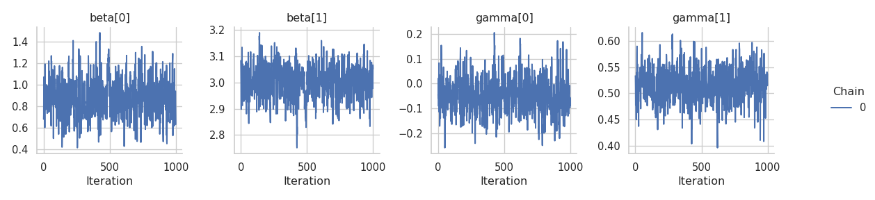
Looks decent although we can see some correlation in the tracplots. Let’s check at the combined summary:

gs.summary_m.Summary(results, per_chain=False)

Parameter summary:

		kernel	mean	sd	q_0.05	q_0.5	q_0.95	sample_size	ess_bulk	ess_tail	rhat
parameter	index
beta	(0,)	kernel_00	0.879	0.183	0.582	0.877	1.185	4000	1784.972	1663.562	1.003
beta	(1,)	kernel_00	3.003	0.064	2.897	3.003	3.104	4000	1912.816	1757.049	1.002
gamma	(0,)	kernel_00	-0.047	0.072	-0.164	-0.047	0.072	4000	1876.328	1934.067	1.001
gamma	(1,)	kernel_00	0.517	0.032	0.464	0.516	0.568	4000	1963.644	1915.291	1.000

Error summary:

				count	relative
kernel	error_code	error_msg	phase
kernel_00	1	divergent transition	warmup	108	0.018
kernel_00	1	divergent transition	posterior	0	0.000

Maybe a longer warm-up would give us better samples.

builder = gs.EngineBuilder(seed=3, num_chains=4)

# connects the engine with the model
builder.set_model(lsl.GooseModel(model))

# we use the same initial values for all chains
builder.set_initial_values(model.state)

# add the kernel
builder.add_kernel(gs.NUTSKernel(["beta", "gamma"]))

# set number of iterations in warmup and posterior
builder.set_duration(warmup_duration=4000, posterior_duration=1000, term_duration=1000)

# create the engine
engine = builder.build()

# generate samples
engine.sample_all_epochs()

liesel.goose.engine - INFO - Starting epoch: FAST_ADAPTATION, 75 transitions, 25 jitted together
liesel.goose.engine - WARNING - Errors per chain for kernel_00: 7, 9, 8, 12 / 75 transitions
liesel.goose.engine - INFO - Finished epoch
liesel.goose.engine - INFO - Starting epoch: SLOW_ADAPTATION, 25 transitions, 25 jitted together
liesel.goose.engine - WARNING - Errors per chain for kernel_00: 2, 2, 2, 2 / 25 transitions
liesel.goose.engine - INFO - Finished epoch
liesel.goose.engine - INFO - Starting epoch: SLOW_ADAPTATION, 50 transitions, 25 jitted together
liesel.goose.engine - WARNING - Errors per chain for kernel_00: 2, 1, 1, 1 / 50 transitions
liesel.goose.engine - INFO - Finished epoch
liesel.goose.engine - INFO - Starting epoch: SLOW_ADAPTATION, 100 transitions, 25 jitted together
liesel.goose.engine - WARNING - Errors per chain for kernel_00: 2, 1, 2, 2 / 100 transitions
liesel.goose.engine - INFO - Finished epoch
liesel.goose.engine - INFO - Starting epoch: SLOW_ADAPTATION, 200 transitions, 25 jitted together
liesel.goose.engine - WARNING - Errors per chain for kernel_00: 4, 4, 2, 5 / 200 transitions
liesel.goose.engine - INFO - Finished epoch
liesel.goose.engine - INFO - Starting epoch: SLOW_ADAPTATION, 400 transitions, 25 jitted together
liesel.goose.engine - WARNING - Errors per chain for kernel_00: 2, 3, 3, 9 / 400 transitions
liesel.goose.engine - INFO - Finished epoch
liesel.goose.engine - INFO - Starting epoch: SLOW_ADAPTATION, 2150 transitions, 25 jitted together
liesel.goose.engine - WARNING - Errors per chain for kernel_00: 7, 10, 5, 7 / 2150 transitions
liesel.goose.engine - INFO - Finished epoch
liesel.goose.engine - INFO - Starting epoch: FAST_ADAPTATION, 1000 transitions, 25 jitted together
liesel.goose.engine - WARNING - Errors per chain for kernel_00: 8, 3, 7, 5 / 1000 transitions
liesel.goose.engine - INFO - Finished epoch
liesel.goose.engine - INFO - Finished warmup
liesel.goose.engine - INFO - Starting epoch: POSTERIOR, 1000 transitions, 25 jitted together
liesel.goose.engine - INFO - Finished epoch

results = engine.get_results()
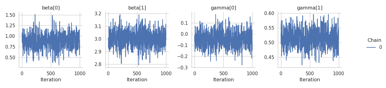
g = gs.plot_trace(results, chain_indices=0, ncol=4)

gs.summary_m.Summary(results, per_chain=False)

Parameter summary:

		kernel	mean	sd	q_0.05	q_0.5	q_0.95	sample_size	ess_bulk	ess_tail	rhat
parameter	index
beta	(0,)	kernel_00	0.880	0.175	0.599	0.880	1.163	4000	1931.337	1504.200	1.004
beta	(1,)	kernel_00	3.002	0.062	2.899	3.003	3.104	4000	1957.767	1619.727	1.003
gamma	(0,)	kernel_00	-0.044	0.071	-0.158	-0.044	0.071	4000	2067.080	2073.264	1.002
gamma	(1,)	kernel_00	0.516	0.031	0.465	0.516	0.567	4000	2167.641	2330.798	1.001

Error summary:

				count	relative
kernel	error_code	error_msg	phase
kernel_00	1	divergent transition	warmup	140	0.009
kernel_00	1	divergent transition	posterior	0	0.000

The trace plots for \(\boldsymbol{\gamma}\) improved but those for \(\boldsymbol{\beta}\) still show some corelation.